Equity valuation basics - Dividend discount and Gordon growth

Learning Outcomes

This article explains core equity valuation techniques using dividend discount approaches, including:

• Applying the dividend discount model (DDM) to value common shares as the present value of expected future dividends.
• Using the Gordon growth (constant growth) model, identifying when its assumptions hold and interpreting its output in exam-style problems.
• Distinguishing clearly between constant, multi-stage, and variable dividend growth patterns and selecting the appropriate model for each.
• Calculating a share’s fundamental value given required return, next-period dividend, and expected growth rate data typically provided in CFA Level 1 questions.
• Deriving an implied required return or implied dividend growth rate from an observed share price using the Gordon growth relation.
• Assessing how small changes in the required rate of return or growth rate affect valuation, and recognizing situations in which the model becomes unstable or invalid (for example, when g ≥ r).
• Identifying and explaining key economic and mathematical assumptions behind DDM and Gordon growth formulations.
• Recognizing limitations of dividend-based valuation for non‑dividend‑paying or high‑reinvestment companies and knowing when alternative valuation approaches are more appropriate.
• Evaluating exam vignettes for common traps, such as inconsistent inputs, inappropriate growth assumptions, incorrect use of D0 vs D1, or misuse of constant‑growth formulas in multi‑stage settings.

CFA Level 1 Syllabus

For the CFA Level 1 exam, you are required to understand equity valuation using dividend discount models, with a focus on the following syllabus points:

• Explain the rationale and formula for valuing equities using the dividend discount model (DDM).
• Describe types of dividends and share repurchases and identify which cash flows are captured by dividend-based valuation models.
• Apply the Gordon growth (constant growth) model and variable/dividend growth approaches, including two-stage and multi-stage models.
• Calculate fundamental value given required return, dividend, and expected growth rate information.
• Calculate and interpret implied required return or implied dividend growth given price and dividend data.
• Analyze the sensitivity of valuation to required return and growth rate assumptions.
• Identify assumptions, limitations, and appropriate use cases of dividend discount models and contrast them with other valuation approaches (for example, multiplier and asset-based models).

Test Your Knowledge

Attempt these questions before reading this article. If you find some difficult or cannot remember the answers, look more closely at that area during your revision.

1. For the Gordon growth model to be valid, which condition must hold?

   • a) The growth rate must be greater than the required return.
   • b) The growth rate must equal the required return.
   • c) The growth rate must be less than the required return and constant.
   • d) Dividends must be zero in the first year.

2. A stock is expected to pay a dividend of $3 next year. Dividends are expected to grow at 4% per year forever, and the required return is 10%. What is the stock’s fundamental value using the Gordon growth model?

   • a) $30.00
   • b) $50.00
   • c) $60.00
   • d) $75.00

3. If the expected constant dividend growth rate g exceeds the required return r in the standard Gordon growth formula, which statement is most accurate?

   • a) The model gives a negative finite value.
   • b) The model gives a very high but still meaningful positive value.
   • c) The model is mathematically unstable and does not produce a meaningful value.
   • d) The model automatically adjusts by lowering the growth rate.

4. Which of the following situations most clearly suggests that a dividend discount model is inappropriate as the primary valuation tool?

   • a) A mature utility company paying stable dividends.
   • b) A bank with a long history of regular cash dividends.
   • c) A fast-growing technology firm that reinvests all earnings and has no plans to pay dividends soon.
   • d) A large manufacturer with a 30-year record of steadily increasing dividends.

Introduction

Dividend-based valuation models are commonly tested on CFA Level 1. The dividend discount model (DDM) provides a framework for valuing a common share as the present value of its future dividends, discounted at the required rate of return. The Gordon growth (constant growth) model is a popular DDM variation, using the assumption of dividends growing at a constant rate in perpetuity. Exam questions often require careful attention to correct inputs, valid model selection, and the implications of growth assumptions.

From a broader standpoint, DDMs are part of the present value family of equity valuation models, which also include free cash flow models. They differ from:

• Multiplier (relative valuation) models: such as price-to-earnings (P/E), where value is inferred by comparing price multiples across securities or to an industry average.
• Asset-based models: where equity value is derived from the estimated market value of assets minus liabilities.

For this article, the focus is on dividend discount models and, in particular, the constant-growth Gordon model.

Key Term: fundamental value
The estimated “true” economic value of a share based on fundamentals (such as expected cash flows and required return), as opposed to its current market price. Key Term: dividend discount model (DDM)
The valuation approach that estimates the fundamental value of a share as the present value of all expected future dividends, discounted at the required rate of return. Key Term: Gordon growth model
A form of the DDM in which future dividends are assumed to grow at a constant rate forever, producing a simplified valuation formula. Key Term: required rate of return (r)
The return equity investors demand given the risks of the share, often estimated using models such as the CAPM; used as the discount rate in valuation. Key Term: perpetual growth
The assumption that cash flows (dividends) will continue indefinitely and increase at a constant rate each period.

Dividend-based models use dividends because they are observable cash distributions to shareholders. In a strictly theoretical sense, even the price at which you hope to sell a share in the future reflects the present value of dividends beyond that date, so dividends ultimately drive value in this framework.

Test Tip: When revising Dividend discount and Gordon growth, connect each definition, method, or rule to the kind of question the assessment is likely to ask.

THE DIVIDEND DISCOUNT MODEL (DDM)

The basic DDM states that the fundamental value of a share today, $V_0$, equals the sum of all expected future dividends $(D_1, D_2, D_3, \ldots)$ discounted back to the present at the required rate of return on equity, $r$:

$V_0 = \sum_{t=1}^{\infty} \frac{D_t}{(1 + r)^t}$

This is just the time value of money applied to equity cash flows. It does not yet impose any particular pattern on dividends; it simply says:

• value = present value of all future dividends.

In practice, you cannot forecast dividends one by one to infinity, so you must impose structure on expected dividend growth.

Dividends and What Counts as a Cash Flow

DDM focuses on cash dividends. To put dividend assumptions in context, recall the main forms of shareholder distributions.

Key Term: regular cash dividend
A recurring cash payment to shareholders (for example, quarterly or annually) that follows a relatively stable pattern. Key Term: extra dividend
A one-off or infrequent cash distribution that supplements (or replaces) regular dividends, often used when earnings are unusually high. Key Term: stock dividend
A dividend paid in additional shares rather than cash; it increases the number of shares outstanding but does not change total shareholder wealth. Key Term: stock split
A proportional increase in the number of shares outstanding (for example, two-for-one split) accompanied by a proportional decrease in share price. Key Term: reverse stock split
A proportional decrease in the number of shares outstanding (for example, one-for-two reverse split) with a proportional increase in share price. Key Term: share repurchase
A transaction in which a company buys back its own shares for cash, reducing shares outstanding and often viewed as an alternative to cash dividends.

For purposes of the basic DDM at Level 1:

• Regular and extra cash dividends are included explicitly as $D_t$.
• Stock dividends and stock splits simply change share count and price proportionally; they do not, by themselves, create or destroy value, so they are not modeled separately in DDM.
• Share repurchases are conceptually similar to dividends (cash returned to shareholders), but the standard DDM focuses on cash dividends only. More advanced models can incorporate repurchases via free cash flow to equity (FCFE), but that is beyond the scope here.

Constant vs. Variable Growth

To use the DDM in calculations, you need an assumption about how dividends change over time.

If dividends are expected to grow at a constant annual rate $g$, starting from some base dividend, we can treat the dividend stream as a growing perpetuity, leading directly to the Gordon growth model.

More often, however, dividend growth is not constant:

• A young firm might have a period of very high growth before maturing.
• A cyclical firm’s dividends might be irregular before stabilizing.
• A turnaround firm might have low or negative growth initially, then recover.

In such cases, analysts typically use multi-stage models:

• Forecast dividends explicitly for a finite period during which growth is non-constant or unusually high or low.
• After that period, assume a constant, sustainable long-term growth rate and apply the Gordon formula to compute a terminal value.

Key Term: multi-stage dividend discount model
A DDM that allows one or more finite stages of non-constant or unusual dividend growth, followed by a perpetual constant-growth stage. Key Term: terminal value
The present value, at the start of the constant-growth stage, of all dividends expected from that point into infinity.

Choosing between constant-growth and multi-stage DDMs is an important judgment point in exam questions.

THE GORDON GROWTH (CONSTANT GROWTH) MODEL

The Gordon growth model values a share as the present value of a perpetual, constantly growing stream of dividends:

$V_0 = \frac{D_1}{r - g}$

Where:

• $V_0$ = fundamental value of the share today
• $D_1$ = expected dividend next year (one period ahead)
• $r$ = required rate of return for equity
• $g$ = expected constant annual growth rate of dividends

It is critical that $D_1$ is the dividend in the next period, not the last dividend paid. If you are given the most recent dividend $D_0$ and a constant growth rate $g$, then:

$D_1 = D_0 (1 + g)$

A common exam trap is to plug $D_0$ directly into the formula instead of $D_1$.

Worked Example 1.1

Suppose a company will pay a dividend of $2.00 per share next year. Dividends are expected to grow at 5% per year indefinitely. The required return is 9%. What is the fair value of the share?

Answer:
Using the Gordon growth model:

$> V_0 = \frac{2.00}{0.09 - 0.05} = \frac{2.00}{0.04} = \$50.00$

If the share trades below $50, it may be undervalued under these assumptions; if it trades above $50, it may be overvalued.

Relation to Expected Return

The Gordon model also gives a useful decomposition of the required return:

$r = \frac{D_1}{P_0} + g$

Where $P_0$ is the current share price. The required return equals:

• a dividend yield component $\left(\frac{D_1}{P_0}\right)$ plus
• a capital growth component $g$.

This relation is often used in reverse to infer either:

• the required return $r$ given $P_0, D_1, g$, or
• the implied constant growth rate $g$ given $P_0, D_1, r$.

Key Term: sustainable growth rate
A long-run dividend (or earnings) growth rate that can be maintained without changing the firm’s capital structure, usually consistent with long-run economic growth and the firm’s reinvestment capacity. Key Term: payout ratio
The fraction of earnings paid out as dividends; dividend per share divided by earnings per share.

At Level 1, you may be given a long-run growth rate directly or asked to compute it from historical data (for example, using a compound annual growth rate) or from a sustainable growth formula in other readings.

Model Assumptions

The Gordon growth model rests on several key assumptions:

• Dividends grow at a constant rate $g$ forever, starting from $D_1$.
• The required return $r$ is constant over time.
• The growth rate is strictly less than the required return: $r > g$.
• The company pays dividends, and dividend policy is reasonably linked to company earnings.

If any of these assumptions is violated, model results can become misleading or mathematically invalid. For instance:

• If dividends are highly irregular or expected to change regimes (for example, high growth to low growth), a multi-stage model is more appropriate.
• If $g \ge r$, the denominator $r - g$ becomes zero or negative, and the formula produces no economically meaningful value.

Worked Example 1.2

A company pays $1.50 per share in expected dividends next year. Analysts forecast dividends will grow at 7% per year. If investors require a 12% return, what is the share's value?

Answer:
Use:

$> V_0 = \frac{D_1}{r - g} = \frac{1.50}{0.12 - 0.07} = \frac{1.50}{0.05} = \$30.00$

Estimating Constant Growth Rates

If you are given beginning and ending dividends over several years and asked to assume constant growth, you can estimate the annual growth rate using a compound growth formula:

$g = \left(\frac{D_{\text{final}}}{D_{\text{initial}}}\right)^{1/N} - 1$

Where:

• $D_{\text{initial}}$ = dividend at the start of the period
• $D_{\text{final}}$ = dividend at the end of the period
• $N$ = number of years between the two dividends

This growth rate can then be used as the constant $g$ in the Gordon model, provided it seems economically realistic.

Implied Return and Implied Growth

Because $r = \frac{D_1}{P_0} + g$, you can infer market expectations:

• Implied required return:

$r = \frac{D_1}{P_0} + g$

• Implied growth rate (given a required return):

$g = r - \frac{D_1}{P_0}$

These manipulations are explicitly tested at Level 1.

Worked Example 1.3

A stock trades at $63.00. The expected dividend next year is $1.89, and dividends are forecast to grow at 4% per year indefinitely. What required return is implied by the current price?

Answer:
First, compute the dividend yield:

> \frac{D_1}{P_0} = \frac{1.89}{63.00} = 0.03 \text{ (3.0%)}

Then add the growth rate:

> r = 0.03 + 0.04 = 0.07 \text{ (7.0%)}

The market price of $63 implies investors require about 7% per year, given these dividend assumptions.

When to Use DDM and the Gordon Model

DDM, and particularly the Gordon growth form, is best suited to:

• Mature, stable companies with predictable dividend patterns (utilities, established consumer staples).
• Firms whose dividend policy closely tracks earnings, such that dividends reasonably represent the cash flows attributable to shareholders.
• Situations where a constant long-run growth rate is a reasonable approximation (for example, large diversified firms growing roughly with the economy).

DDM is less suitable when:

• The company does not pay dividends and has no credible plan to initiate them in the foreseeable future.
• Dividends are highly irregular, suspended, or driven by one-off events.
• Reinvestment opportunities are very attractive, and dividends are intentionally kept low so that value shows up mainly as price appreciation, not dividends.

Worked Example 1.4

ABC Corp. does not pay dividends and has no plans to initiate dividends for at least 5 years. Is the DDM appropriate for ABC Corp. valuation?

Answer:
No. The DDM assumes dividends drive valuation. For companies not paying dividends (and with no expectation to pay in the foreseeable future), the present value of dividends is zero under current assumptions. Alternative models—such as discounted free cash flow to equity, or price multiple comparisons—are more appropriate.

Multi-Stage Dividend Growth Models

Many companies experience an initial period of high or unstable growth before settling into a lower, sustainable growth rate. In these cases, analysts use multi-stage models.

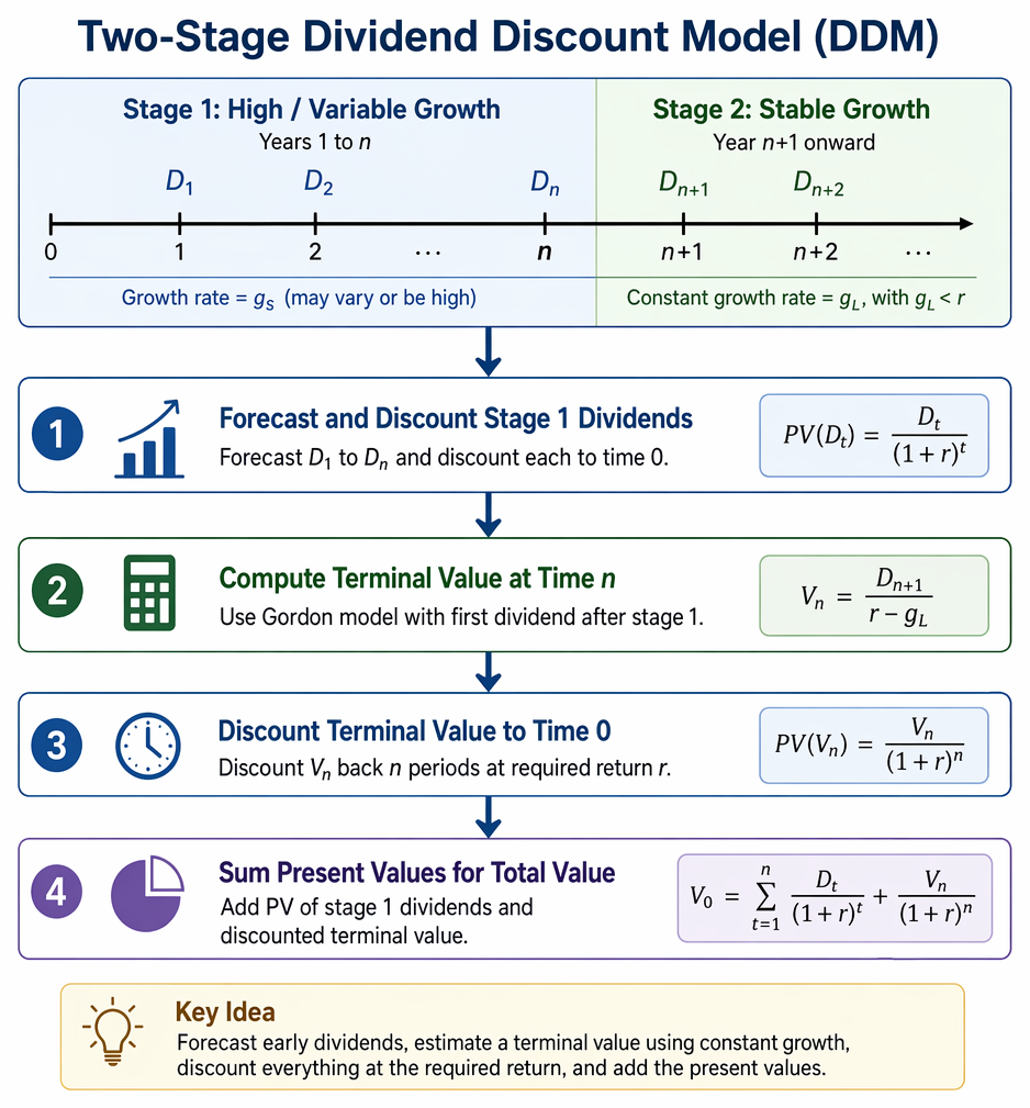
Equity valuation under the DDM is shown as forecasting dividends, assessing constant sustainable growth, and deriving present value from the model.

The basic two-stage DDM works as follows:

• Stage 1: Dividends grow at a higher or non-constant rate $g_S$ for $n$ years.
• Stage 2: After year $n$, dividends grow at a constant long-run rate $g_L$, with $g_L < r$.

The valuation procedure is:

• Forecast and discount each dividend in stage 1.

• At the end of stage 1 (time $n$), compute the terminal value using the Gordon model:

  $V_n = \frac{D_{n+1}}{r - g_L}$

• Discount $V_n$ back to time 0 and add to the present value of stage 1 dividends.

Worked Example 1.5

Suppose Beta Inc. will pay dividends as follows: D_1 = \1.00$,$D_2 = $1.15$,$D_3 = $1.30$. After year 3, dividends will grow at 4% per year forever. The required return is 10%. What is the value of the share today?

Answer:
Step 1: Discount year 1–3 dividends:

$> \text{PV}_{D1} = \frac{1.00}{1.10^1} = 0.909$

$> \text{PV}_{D2} = \frac{1.15}{1.10^2} = 0.950$

$> \text{PV}_{D3} = \frac{1.30}{1.10^3} = 0.975$

Step 2: Compute the terminal value at $t = 3$. First find $D_4$:

$> D_4 = 1.30 \times 1.04 = 1.352$

Then:

$> TV_3 = \frac{D_4}{r - g} = \frac{1.352}{0.10 - 0.04} = 22.53$

Discount the terminal value to today:

$> \text{PV}_{TV} = \frac{22.53}{1.10^3} = 16.98$

Step 3: Sum all present values:

$> V_0 = 0.909 + 0.950 + 0.975 + 16.98 \approx \$19.81$

In the exam, the structure is similar even if:

• Stage 1 is defined by a growth rate $g_S$ rather than specific dividend amounts, or
• There are more than two stages (for example, high growth, transition, and stable growth).

The core steps are always:

• Forecast dividends.
• Compute terminal value using a constant-growth assumption.
• Discount all cash flows at the required return.

Valuing a Stock with No Dividends for Several Years

Sometimes a firm currently pays no dividend, but is expected to initiate dividends later and then grow at a constant rate. You can still use the Gordon model by:

• Valuing the stock at the time just before dividends start (using the first positive dividend and constant growth assumptions).
• Discounting that value back to today.

Worked Example 1.6

A company pays no dividends now but is expected to pay its first dividend of $4.00 four years from today (at $t = 4$). From that point, dividends are expected to grow at 6% per year indefinitely. The required return is 10%. What is the fundamental value today?

Answer:
Method: First find the value at $t = 3$ or $t = 4$, then discount to today. Viewpoint at $t = 3$: At time 3, the next dividend (one year ahead) is $D_4 = 4.00$. Dividends grow at 6% thereafter. Use the Gordon model at $t = 3$:

$> V_3 = \frac{D_4}{r - g} = \frac{4.00}{0.10 - 0.06} = \frac{4.00}{0.04} = 100.00$

Discount $V_3$ three years back to today:

$> V_0 = \frac{100.00}{1.10^3} \approx 75.13$

So the estimated fundamental value today is about $75.13, even though dividends are zero for the first three years.

This technique is needed when the problem specifies dividends start in the future but then grow at a constant rate.

Exam Warning: The Gordon growth model only applies if $r > g$. If you are given values where $g \geq r$, the model produces nonsensical or infinite valuations—an easy exam trap.

Additional practical exam cautions:

• Check you are using $D_1$, not $D_0$, in the formula.
• Ensure $r$ and $g$ are in the same units (for example, both nominal annual rates).
• Verify that your long-run growth rate is economically plausible (for large firms, long-run growth much higher than GDP growth is usually unrealistic).

If any assumption looks unreasonable, consider whether a multi-stage model or alternative valuation approach is implied by the vignette.

Sensitivity to Growth and Required Return

The DDM, especially the Gordon model, is highly sensitive to small changes in $g$ and $r$, because both appear in the denominator as $r - g$.

Key Term: sensitivity analysis
The process of examining how model outputs (for example, share value) change when key assumptions (such as $r$ or $g$) are varied.

Consider a simple illustration. Suppose the most recent dividend was $2.50, and dividends are expected to grow at 5% forever. The required return is initially estimated at 9%.

1. Compute $D_1 = 2.50 \times 1.05 = 2.625$.

2. Base-case value:

   $V_0 = \frac{2.625}{0.09 - 0.05} = \frac{2.625}{0.04} = 65.63$

Now suppose an analyst revises assumptions modestly:

• growth lowered to 4%,
• required return increased to 10%.

1. New $D_1 = 2.50 \times 1.04 = 2.60$.

2. New value:

   $V_0 = \frac{2.60}{0.10 - 0.04} = \frac{2.60}{0.06} \approx 43.33$

A small change in assumptions (growth down 1%, required return up 1%) reduces the value estimate by more than 30%. Exam questions may ask you to:

• compare valuations under different $r$ and $g$;
• identify which assumption (growth vs required return) the model is more sensitive to;
• recognize when the model is unstable (for example, $r$ only slightly above $g$).

Understanding this sensitivity is important for interpreting answer choices and for qualitative questions about model limitations.

Limitations of Dividend Discount Models

Although DDMs are theoretically appealing, they have practical limitations:

• Dividend relevance: Not all companies pay dividends, and even when they do, dividends may not reflect the firm’s full earning power (for example, due to share repurchases or retention for investment).
• Forecasting difficulty: Long-term dividend growth is inherently uncertain. Misestimating $g$ significantly distorts valuations.
• Model sensitivity: As illustrated, small changes in $r$ or $g$ can produce large changes in estimated value, especially when $r - g$ is small.
• Inapplicability to certain firms: High-growth, early-stage, or distressed firms may not have meaningful or predictable dividend patterns.
• Over-simplicity of constant growth: The assumption of one constant growth rate forever often does not capture realistic life cycles of firms.

When DDMs are unsuitable, analysts often turn to:

• Free cash flow models (that is, discounting free cash flow to equity or to the firm).
• Multiplier models (for example, P/E, price-to-book, or enterprise-value-to-EBITDA).
• Asset-based approaches in asset-heavy businesses or liquidation contexts.

At Level 1, you should be able to identify when a DDM (especially the Gordon form) is appropriate and when it is not.

Summary

Dividend discount models value shares as the present value of future expected dividends, discounted at the required rate of return. The Gordon growth model provides a simple, closed-form solution when dividends grow at a constant rate forever and the required return exceeds the growth rate.

When growth is not constant, analysts apply multi-stage DDMs: forecast dividends explicitly during non-constant growth periods, compute a terminal value using the Gordon model at the start of the constant-growth stage, and discount all cash flows back to the present.

Key skills for CFA Level 1 include:

• recognizing when constant-growth assumptions are reasonable;
• correctly applying the Gordon formula (including using $D_1$ and ensuring $r > g$);
• handling multi-stage scenarios with explicit dividend forecasts and terminal values;
• deriving implied required returns or growth rates from current prices; and
• understanding the sensitivity and limitations of dividend-based valuation.

Key Point Checklist

This article has covered the following key knowledge points:

• Apply the general DDM to express equity value as the present value of expected future dividends.
• Use the Gordon growth (constant growth) model and understand its formula, including the requirement that $r > g$ and that $D_1$ is used.
• Distinguish between constant, two-stage, and multi-stage dividend growth patterns and select the appropriate model for each.
• Calculate fundamental value given expected dividend, growth rate, and required return, including cases where dividends start in the future.
• Derive implied required return or implied dividend growth from observed price and dividend data.
• Perform simple sensitivity analysis on DDM valuations with respect to changes in $r$ and $g$.
• Recognize the economic and mathematical assumptions of DDM and Gordon models.
• Identify limitations of dividend discount models and know when alternative valuation methods are more appropriate.
• Avoid common exam traps, such as using $D_0$ instead of $D_1$ or applying the constant-growth model when growth is clearly changing.

Key Terms and Concepts

• fundamental value
• dividend discount model (DDM)
• Gordon growth model
• required rate of return (r)
• perpetual growth
• regular cash dividend
• extra dividend
• stock dividend
• stock split
• reverse stock split
• share repurchase
• multi-stage dividend discount model
• terminal value
• sustainable growth rate
• payout ratio
• sensitivity analysis