Probability and sampling - Sampling estimation and confidence intervals

Learning Outcomes

This article explains how probability-based measures and sampling-based inference are used in the CFA Level 1 curriculum for rigorous investment analysis, including:

• Interpreting and computing expected value, variance, and standard deviation for asset returns and portfolios.
• Distinguishing populations, parameters, samples, statistics, and point estimates in typical investment data settings.
• Comparing probability and non-probability sampling methods, and evaluating their impact on estimator reliability.
• Explaining sampling error, standard error, and the sampling distribution of the sample mean in detail.
• Applying the central limit theorem to justify normal or t-based inference for means in practice.
• Constructing, interpreting, and comparing confidence intervals for a population mean across common exam-style scenarios.
• Assessing how sample size, variability, confidence level, and distributional assumptions affect interval width and precision.
• Recognizing major sampling-related biases that distort estimates, such as survivorship, look-ahead, and data-snooping bias.
• Linking confidence intervals to hypothesis testing logic used in the curriculum to evaluate investment claims.

CFA Level 1 Syllabus

For the CFA Level 1 exam, you are required to understand probability theory and its applications to investment analysis, with a focus on the following syllabus points:

• The meaning and calculation of expected value, variance, and standard deviation of a random variable
• The distinction between populations, samples, parameters, and statistics
• Sampling methods (simple random, stratified random, cluster, convenience, judgmental)
• The concept of sampling error and the sampling distribution of a statistic
• The central limit theorem and its implications for the distribution of the sample mean
• Confidence interval construction for population parameters based on sample statistics
• Effects of sample size, distributional assumptions, and biases on inference and confidence

Test Your Knowledge

Attempt these questions before reading this article. If you find some difficult or cannot remember the answers, look more closely at that area during your revision.

1. The expected value of a discrete random variable is best described as:

   • a) The most frequently occurring outcome in the distribution
   • b) The simple arithmetic average of observed outcomes in a sample
   • c) The probability‑weighted average of all possible outcomes
   • d) The median of the distribution

2. Which sampling method guarantees that every element of the population has a known, non‑zero probability of selection?

   • a) Convenience sampling
   • b) Judgmental sampling
   • c) Simple random sampling
   • d) Quota sampling

3. According to the central limit theorem, as sample size increases, the sampling distribution of the sample mean:

   • a) Becomes uniform regardless of the population distribution
   • b) Becomes approximately normal with variance equal to σ²n
   • c) Becomes approximately normal with variance equal to σ²⁄n
   • d) Remains identical to the population distribution

4. To construct a 95% confidence interval for a population mean with unknown variance based on a small sample from a normal population, you should use:

   • a) The sample mean and a z‑statistic with σ
   • b) The sample mean and a t‑statistic with s
   • c) The population mean and a t‑statistic with σ
   • d) The sample median and a z‑statistic with s

Introduction

Probability and sampling are fundamental for drawing objective and accurate conclusions from data, particularly in investment analysis. Analysts rarely observe the entire population of returns for an asset or strategy; they usually see only a sample (for example, 60 monthly returns). Understanding how to estimate population parameters from a sample and quantify uncertainty with confidence intervals is critical for interpreting investment performance and risk.

Key Term: population
The complete set of all possible observations of interest, such as all future monthly returns on an index or all firms in a given market. Key Term: sample
A subset of the population used to calculate statistics and make inferences about population parameters. Key Term: parameter
A numerical characteristic of a population (for example, the true population mean or variance) that is usually unknown and must be estimated. Key Term: statistic
A numerical characteristic calculated from sample data (for example, sample mean or sample variance) used to estimate a corresponding population parameter.

In this context, probability describes uncertain future returns, sampling describes how we obtain data, and estimation and confidence intervals describe how we convert that data into statements about parameters such as expected return and risk.

Test Tip: When revising Sampling estimation and confidence intervals, connect each definition, method, or rule to the kind of question the assessment is likely to ask.

Expected Value and Variance

The expected value of a random variable is its long‑run average outcome, weighted by the probabilities of each value. In investment analysis, this is often interpreted as the expected return on a security or portfolio.

Key Term: random variable
A variable whose possible values are outcomes of a random process, each associated with a probability (for example, next year’s return on a stock). Key Term: expected value
The probability‑weighted average value of all possible outcomes of a random variable.

For a discrete random variable X that can take values x₁, x₂, …, xₙ with probabilities p₁, p₂, …, pₙ, the expected value is:

$E(X) = \sum_{i=1}^{n} x_i p_i$

Variance and standard deviation measure dispersion around this expected value.

Key Term: variance
The probability‑weighted average of the squared deviations of each outcome from the expected value; a measure of dispersion. Key Term: standard deviation
The square root of the variance, measuring dispersion in the same units as the original variable.

For a discrete random variable X:

$\text{Var}(X) = \sum_{i=1}^{n} [x_i - E(X)]^2 p_i$

Standard deviation is √Var(X).

In portfolio analysis:

• Expected return measures the central tendency of returns.
• Variance and standard deviation measure risk (volatility of returns).
• These population quantities are usually unknown and must be estimated from sample data.

Because we typically observe only a finite sample of returns, we compute sample counterparts:

$\bar{X} = \frac{1}{n} \sum_{i=1}^{n} X_i, \quad s^2 = \frac{\sum_{i=1}^{n} (X_i - \bar{X})^2}{n-1}$

Here, $\bar{X}$ and $s^2$ are statistics used as point estimates of the population mean μ and variance σ².

Point Estimation and Properties of Estimators

Key Term: point estimate
A single numerical value calculated from sample data used as an estimate of a population parameter. Key Term: estimator
The formula or rule used to compute a point estimate from sample data (for example, the sample mean formula).

Because a statistic depends on which sample is drawn, it is itself a random variable with its own distribution, called a sampling distribution.

Key Term: sampling distribution
The probability distribution of all possible values of a statistic computed from repeated random samples of the same size from the same population.

For example, if you repeatedly sample 12 monthly returns from an equity index and compute the sample mean each time, the distribution of these sample means is the sampling distribution of $\bar{X}$.

Desirable properties of estimators at Level 1 include:

Key Term: unbiased estimator
An estimator whose expected value equals the parameter it estimates.

• The sample mean $\bar{X}$ is an unbiased estimator of μ.
• The sample variance $s^2$ with denominator n – 1 is an unbiased estimator of σ².

Key Term: efficiency
For two unbiased estimators of the same parameter, the more efficient estimator has a smaller variance of its sampling distribution. Key Term: consistency
An estimator is consistent if it converges in probability to the true parameter as sample size increases (its sampling distribution becomes more concentrated around the true value).

At Level 1 you are mainly expected to recognize these properties conceptually and understand that using standard formulas (like $\bar{X}$ and $s^2$ with n – 1) gives estimators with good properties under standard assumptions.

Sampling Methods and Sampling Error

A sample is a subset of a population used to make inferences about parameters such as the population mean or variance. Sampling methods determine how well the sample represents the population and what errors may arise.

Key Term: simple random sampling
A probability sampling method where each member of the population has an equal and independent probability of being selected. Key Term: stratified random sampling
A probability sampling method where the population is divided into subgroups (strata) based on key characteristics, and random samples are drawn from each stratum in proportion to its size. Key Term: cluster sampling
A probability sampling method where the population is divided into clusters that are mini‑populations; entire clusters (and possibly subsamples within them) are randomly selected. Key Term: convenience sampling
A non‑probability sampling method where elements are selected because they are easily accessible to the researcher. Key Term: judgmental sampling
A non‑probability sampling method where elements are deliberately selected based on the researcher’s knowledge and professional judgment.

Probability sampling (simple random, stratified, cluster):

• Allows use of probability theory (like the central limit theorem).
• Supports unbiased estimation and valid measures of sampling error.

Non‑probability sampling (convenience, judgmental):

• Can be faster and cheaper.
• Typically does not support formal probability‑based inference; the sample may not be representative.

Key Term: sampling error
The difference between a sample statistic and the corresponding population parameter, arising because only a subset of the population is observed.

Sampling error is unavoidable when using samples, but appropriate sampling design and larger sample sizes can reduce its magnitude.

Sampling Error and the Standard Error

The variability of a statistic across samples is summarized by its standard error.

Key Term: standard error
The standard deviation of the sampling distribution of a statistic; often estimated from sample data and used in confidence interval construction.

For the sample mean:

• If population standard deviation σ is known:

$\text{Standard error of } \bar{X} = \frac{\sigma}{\sqrt{n}}$

• If σ is unknown, we estimate it using the sample standard deviation s:

$\text{Estimated standard error of } \bar{X} = \frac{s}{\sqrt{n}}$

Notice that as n increases, the standard error decreases: sample means from larger samples fluctuate less around μ.

Simple Random vs Stratified Random vs Cluster Sampling (Investment Examples)

• Simple random sampling: Choose 100 stocks at random from a broad equity universe to estimate the average dividend yield.
• Stratified random sampling: Divide the bond market into strata by maturity, credit rating, and sector; randomly select bonds within each stratum in proportion to its market weight to construct an indexed bond portfolio.
• Cluster sampling: Divide individual investors geographically by state, randomly select several states (clusters), then survey randomly chosen investors within those states about their risk tolerance.

Stratified sampling often gives more precise estimates (smaller variance) than simple random sampling when the strata are more homogeneous internally and differ across groups.

The Central Limit Theorem

One of the most powerful results in statistics for Level 1 is the central limit theorem (CLT). It justifies using normal‑based methods even when the population is not normal.

Key Term: central limit theorem
For a population with mean μ and finite variance σ², the sampling distribution of the sample mean

$> \bar{X}$

from random samples of size n becomes approximately normal with mean μ and variance σ²⁄n as n becomes large.

Key implications:

• For large n (often n ≥ 30 is used as a rule of thumb), $\bar{X}$ is approximately normally distributed, regardless of the shape of the population distribution (provided variance is finite).
• The mean of the sampling distribution of $\bar{X}$ is μ.
• The variance of the sampling distribution of $\bar{X}$ is σ²⁄n, so its standard deviation (standard error) is σ⁄√n.

This allows analysts to:

• Use z‑statistics and normal‑based confidence intervals for means when n is large, even if returns themselves are skewed or heavy‑tailed.
• Rely on sample means becoming more stable and predictable as more observations are collected.

However, for small samples (n < 30) from non‑normal populations, the CLT may not provide a good approximation; special care is required, and t‑based methods formally require a normal population.

Confidence Intervals for the Population Mean

When estimating a population parameter such as the mean from a sample, it is important to quantify uncertainty. Confidence intervals provide a probabilistic range in which the true population parameter is likely to lie.

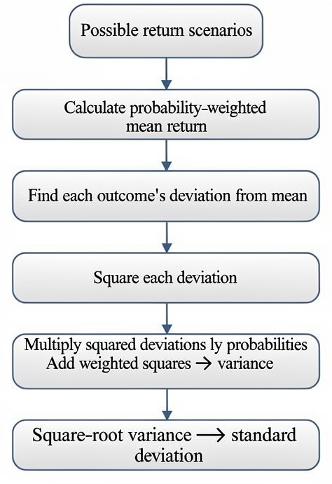
Possible return outcomes and probabilities are processed sequentially to obtain expected value, variance, and standard deviation.

Key Term: confidence interval
A range of values, derived from a sample statistic, that is likely to contain the population parameter with a specified probability (for example, 95%).

Interpretation:

• Probabilistic interpretation: In repeated sampling, 95% of all 95% confidence intervals constructed in the same way will contain the true parameter.
• Practical interpretation: For the single interval you compute, you say you are “95% confident” it contains the true parameter, based on that long‑run property.

The generic structure of a two‑sided confidence interval is:

$\text{Point estimate} \pm \text{Reliability factor} \times \text{Standard error}$

Key Term: reliability factor
A critical value from the assumed sampling distribution (z or t) that determines how many standard errors to extend on each side of the point estimate for a chosen confidence level.

Common reliability factors for the standard normal (z) distribution:

• 90% confidence: z₀.₀₅ ≈ 1.65
• 95% confidence: z₀.₀₂₅ ≈ 1.96
• 99% confidence: z₀.₀₀₅ ≈ 2.58

As the confidence level increases (for example, from 90% to 99%), the reliability factor increases and the interval becomes wider (less precise).

Choosing Between z and t

Key Term: t-distribution
A bell‑shaped distribution similar to the normal but with heavier tails, used when estimating a mean with unknown variance from a normal population, especially with small samples. Key Term: degrees of freedom
The number of independent pieces of information used to estimate a parameter; for a sample variance and t‑based mean, degrees of freedom are n – 1.

For a confidence interval for the population mean μ, three practical cases are examined at Level 1:

1. Population variance known, normal population (any n) or large n by CLT

   $\bar{X} \pm z_{\alpha/2} \frac{\sigma}{\sqrt{n}}$

2. Population variance unknown, normal population, small sample (n < 30)

   Use the t‑distribution with n – 1 degrees of freedom:

   $\bar{X} \pm t_{\alpha/2,\,n-1} \frac{s}{\sqrt{n}}$

3. Population variance unknown, large sample (n ≥ 30)

   Two approaches are acceptable:

   • Normal (z‑based) “alternative”:

   $\bar{X} \pm z_{\alpha/2} \frac{s}{\sqrt{n}}$

   • t‑based interval with n – 1 degrees of freedom; for large n, t and z critical values are very close, and t is slightly more conservative (wider).

Worked Example 1.1

A sample of 64 equity returns has a sample mean of 8% and a known population standard deviation of 12%. Construct a 95% confidence interval for the population mean return.

Answer:
Standard error = 12% ÷ √64 = 12% ÷ 8 = 1.5%. For 95% confidence and known σ, use z₀.₀₂₅ = 1.96. Half‑width = 1.96 × 1.5% = 2.94%. Confidence interval = 8% ± 2.94% = [5.06%, 10.94%]. Interpretation: You are 95% confident that the true mean return lies between 5.06% and 10.94%.

Worked Example 1.2

A financial analyst samples 20 hedge funds and calculates a mean annual return of 9% with a sample standard deviation of 8%. Assume returns are approximately normal. Construct a 90% confidence interval for the population mean.

Answer:
Population variance is unknown and n = 20 (< 30), so use the t‑distribution with n – 1 = 19 degrees of freedom. Estimated standard error = 8% ÷ √20 ≈ 8% ÷ 4.472 ≈ 1.79%. For 90% confidence and 19 df, t₀.₀₅,₁₉ ≈ 1.729. Half‑width = 1.729 × 1.79% ≈ 3.1%. Confidence interval = 9% ± 3.1% ≈ [5.9%, 12.1%]. Interpretation: You are 90% confident that the mean annual return of the hedge fund population lies between 5.9% and 12.1%.

Worked Example 1.3

An analyst computes Sharpe ratios for a random sample of 100 US equity mutual funds. The sample mean Sharpe ratio is 0.45 with a sample standard deviation of 0.30. Construct a 90% confidence interval for the population mean Sharpe ratio.

Answer:
Population variance is unknown, but n = 100 is large, so a z‑based interval is acceptable. Estimated standard error = 0.30 ÷ √100 = 0.03. For 90% confidence, z₀.₀₅ = 1.65. Half‑width = 1.65 × 0.03 = 0.0495. Confidence interval = 0.45 ± 0.0495 ≈ [0.4005, 0.4995], which is often rounded to [0.40, 0.50]. The analyst can say with 90% confidence that the mean Sharpe ratio for the population of similar US equity mutual funds lies between 0.40 and 0.50.

Confidence Intervals and Hypothesis Tests

Confidence intervals are closely related to two‑sided hypothesis tests about the mean. For example, a 95% confidence interval for μ is:

$\bar{X} \pm 1.96 \frac{\sigma}{\sqrt{n}}$

Testing $H_0: \mu = \mu_0$ at the 5% significance level (two‑sided) using a z‑test is equivalent to checking whether μ₀ lies inside the 95% confidence interval:

• If μ₀ lies outside the interval, reject H₀.
• If μ₀ lies inside the interval, fail to reject H₀.

This equivalence is often tested conceptually at Level 1.

Sample Size Selection and Interval Width

Analysts often want their estimate to be within a specified margin of error E of the true mean, with given confidence. For a z‑based interval with known σ, solving

$E = z_{\alpha/2} \frac{\sigma}{\sqrt{n}}$

for n gives:

$n = \left(\frac{z_{\alpha/2} \, \sigma}{E}\right)^2$

Main effects on interval width:

• Higher confidence level (larger reliability factor) → wider interval.
• Higher population variability (larger σ) → wider interval.
• Larger sample size n → smaller standard error → narrower interval.

Worked Example 1.4

Question: Suppose the annual standard deviation of a portfolio’s returns is believed to be 16%. How large a sample of annual returns is needed to estimate the mean return with a margin of error of ±2% at the 95% confidence level (assume σ known)?

Answer:
Desired margin of error E = 2% = 0.02. σ = 16% = 0.16. For 95% confidence, z₀.₀₂₅ = 1.96. Required sample size:

$> n = \left(\frac{1.96 \times 0.16}{0.02}\right)^2 = \left(\frac{0.3136}{0.02}\right)^2 = (15.68)^2 \approx 245$

So, approximately 245 annual observations are needed. In practice, you would round up to at least 245 years (which is usually not feasible), illustrating that for annual data, tight margins of error require very long series. With monthly or daily data, reaching a similar n is more achievable.

Practical Considerations in Inference

Several practical issues affect the validity and usefulness of sampling‑based inference in finance.

Distributional Assumptions and Small Samples

• Many methods (t‑based intervals for means) assume the population is normal.
• With small samples (n < 30), this assumption is important. If returns are highly skewed or heavy‑tailed, a t‑interval may not have the advertised coverage probability.
• With large samples, the central limit theorem often makes the sample mean approximately normal even if returns themselves are not.

Outliers and Non‑stationarity

• Financial return series may contain outliers (extreme events) or structural breaks (e.g., regime changes).
• Outliers increase the sample standard deviation and widen confidence intervals.
• If the process is not stable over time (non‑stationary), older data may not be representative of current conditions; this affects the interpretation of any interval estimate.

Sampling‑Related Biases

Key Term: sampling bias
A systematic error in a sample that causes it to misrepresent the population, leading to biased estimates and misleading inference.

Key sampling‑related biases covered in the CFA curriculum:

Key Term: data snooping bias
Bias arising from repeatedly searching the same dataset for patterns or strategies and reporting only the successful findings, which may be due to chance. Key Term: sample selection bias
Bias arising when the procedure for selecting sample observations excludes certain members of the population in a systematic way. Key Term: survivorship bias
A form of sample selection bias where only surviving entities (for example, funds or companies that still exist) are included, overstating historical performance. Key Term: look-ahead bias
Bias arising when a study uses information that would not have been available at the time decisions were made. Key Term: time-period bias
Bias arising when results are sensitive to the specific time period examined (for example, including or excluding major crises).

These biases affect both point estimates and confidence intervals:

• Data snooping can produce apparently significant results that do not hold out of sample.
• Survivorship bias can make average returns and Sharpe ratios look higher than they truly are.
• Look‑ahead bias can make trading rules appear profitable using information that real‑time investors did not have.
• Time‑period bias can lead to over‑ or underestimation of risk and return if the period is unusually strong or weak.

For the exam, you should be able to recognize these biases conceptually and understand that they undermine the reliability of statistical inference.

Exam Warning: Exam warning: For n < 30 and unknown population variance, and when the population is (or is stated to be) normal, always use the t‑distribution and the sample standard deviation to construct a confidence interval for the mean. Using a z‑statistic in this setting is a common error.

Another common mistake is misinterpreting the confidence level. A 95% confidence interval does not mean there is a 95% chance that μ lies within the calculated interval after observing the data; rather, it describes the long‑run performance of the interval‑construction procedure.

Summary

Probability and sampling provide the basis for statistical inference in finance. The expected value and variance of a random variable describe the long‑run average return and its dispersion, forming the basis of risk–return analysis. Because analysts typically do not observe entire populations, they work with samples and use sample statistics as estimators of population parameters.

Understanding how samples are collected (simple random, stratified random, cluster, convenience, judgmental) is essential because sampling error and sampling bias directly affect the reliability of estimates. The central limit theorem justifies approximating the sampling distribution of the sample mean by a normal distribution for large samples, enabling the use of z‑ and t‑based confidence intervals.

Confidence intervals quantify the uncertainty around point estimates of the population mean, with their width driven by variability, sample size, and the chosen confidence level. Recognizing when to use the normal vs t‑distribution, how to interpret reliability factors and degrees of freedom, and how sample size influences precision are all key skills for CFA Level 1.

Finally, awareness of practical limitations—such as non‑normality, small samples, outliers, and sampling‑related biases—helps you interpret statistical results more cautiously and avoid typical exam pitfalls.

Key Point Checklist

This article has covered the following key knowledge points:

• Interpret and calculate expected value, variance, and standard deviation of a random variable.
• Distinguish populations, samples, parameters, and statistics in investment contexts.
• Understand estimators, point estimates, and properties such as unbiasedness, efficiency, and consistency.
• Identify and compare sampling methods (simple random, stratified random, cluster, convenience, judgmental) and their implications.
• Explain the meaning of sampling error and the role of the sampling distribution and standard error.
• Apply the central limit theorem to justify normal approximations for the sampling distribution of the mean.
• Construct and interpret confidence intervals for a population mean using z‑ and t‑distributions in appropriate settings.
• Explain how confidence level, population variability, and sample size affect the width of confidence intervals.
• Relate confidence intervals to two‑sided hypothesis tests about the mean.
• Recognize major sampling‑related biases (data snooping, sample selection, survivorship, look‑ahead, time‑period) and their impact on inference.

Key Terms and Concepts

• population
• sample
• parameter
• statistic
• random variable
• expected value
• variance
• standard deviation
• point estimate
• estimator
• sampling distribution
• unbiased estimator
• efficiency
• consistency
• simple random sampling
• stratified random sampling
• cluster sampling
• convenience sampling
• judgmental sampling
• sampling error
• standard error
• central limit theorem
• confidence interval
• reliability factor
• t-distribution
• degrees of freedom
• sampling bias
• data snooping bias
• sample selection bias
• survivorship bias
• look-ahead bias
• time-period bias