Learning Outcomes
This article explains credit risk measurement and portfolio strategies for the CFA Level 2 exam, including:
- Quantifying and interpreting credit risk at the instrument and portfolio level using PD, LGD, and EAD.
- Computing expected loss, decomposing its drivers, and assessing the sensitivity of EL to changes in PD, LGD, and EAD.
- Applying credit migration (transition) matrices to estimate default and rating-change losses, and to distinguish between point-in-time PDs, hazard rates, and multi-period (cumulative) default probabilities.
- Incorporating recovery rate assumptions, collateral, and seniority into LGD estimates and loss projections.
- Estimating and interpreting credit valuation adjustment (CVA) for loans, bonds, and derivative or bilateral exposures.
- Linking credit-risk metrics to pricing, capital allocation, diversification, concentration limits, and portfolio strategy decisions.
- Performing exam-style numerical calculations and avoiding common pitfalls such as confusing cumulative and marginal PDs, ignoring survival probabilities, or mis-specifying EAD.
- Comparing credit risk across instruments and portfolios using expected loss, migration-based measures, and CVA-based valuation.
CFA Level 2 Syllabus
For the CFA Level 2 exam, you are required to understand the quantitative assessment of credit risk within a portfolio context, with a focus on the following syllabus points:
- Explain and calculate expected loss, loss given default (LGD), exposure at default (EAD), and probability of default (PD).
- Use credit migration (transition) matrices to estimate portfolio credit risk and expected loss.
- Describe the use of LGD and credit migration in credit valuation adjustment (CVA).
- Analyze the impact of credit risk metrics on portfolio strategies and risk management approaches.
- Compare credit-risk measures across instruments using expected loss and related quantities.
Test Your Knowledge
Attempt these questions before reading this article. If you find some difficult or cannot remember the answers, look more closely at that area during your revision.
Delta Bank is assessing the credit risk of a new one-year lending relationship with Alpha Co. The bank considers both direct lending and a derivative exposure to the same counterparty. The analyst has gathered the following information:
- Proposed term loan: notional $5 million, one-year PD of 1.5%, expected recovery rate 40%.
- Unused revolving credit facility: committed but undrawn amount $2 million. For capital purposes, the bank assumes that 50% of the undrawn amount will be drawn at the time of default.
- A one-year interest rate swap with Alpha Co. is expected to have an average positive exposure over the year of $0.8 million. For simplicity, the analyst uses a one-year PD of 1.5% and LGD of 60% for the swap.
- The bank also has access to a one-year transition matrix for Alpha’s current rating (A), which shows a 2% probability of downgrade to BBB, 1.5% probability of downgrade to BB, and 0.5% probability of default over one year.
Using this information, answer the following:
-
What is the best estimate of Delta Bank’s total one-year expected loss on the Alpha relationship, using the standard EL formula and the given assumptions?
- a) $45,000
- b) $72,000
- c) $81,000
- d) $99,000
-
Suppose credit conditions deteriorate and Alpha’s one-year PD is revised upward to 3% while LGD and EAD assumptions remain unchanged. How will the total expected loss on the Alpha relationship change?
- a) It will increase, approximately doubling because expected loss is proportional to PD.
- b) It will increase, but by less than 50% because exposure is partially drawn.
- c) It will remain unchanged because LGD and EAD are unchanged.
- d) It will decrease if Delta reduces the loan coupon to compensate for the higher PD.
-
Which statement best describes the role of the credit migration (transition) matrix in expected loss estimation for Alpha’s bond or loan?
- a) It is used only to estimate the one-year default probability; all non-default transitions are irrelevant for credit risk.
- b) It provides probabilities of all rating changes, allowing the analyst to estimate both default losses and mark-to-market losses from rating downgrades.
- c) It is used to compute the effective duration of the bond and has no direct implication for expected loss.
- d) It is relevant only for equity investors because rating migration affects equity volatility, not credit losses.
-
Which of the following is the most accurate definition of loss given default (LGD) from Delta Bank’s standpoint?
- a) The probability that Alpha Co. will default within a given year.
- b) The average annual interest income lost if Alpha’s credit rating is downgraded.
- c) The percentage of EAD that the bank does not expect to recover if Alpha defaults.
- d) The present value of all expected coupon payments discounted at a risk-free rate.
Introduction
Credit risk management requires understanding the components and calculation of expected loss for individual credit exposures and portfolios. This includes quantifying the likelihood and severity of losses due to default events, measuring risk with inputs such as probability of default, exposure at default, loss given default, and interpreting the effect of credit migration. You must be able to use these measures to estimate portfolio risk, inform allocation, and support disciplined credit portfolio strategies.
At Level 2, you are expected not only to know the definitions, but to apply them across different instruments (loans, bonds, derivatives), time horizons, and credit states. In practice, expected loss is computed over multiple periods using conditional default probabilities and time-varying exposures; exam questions often simplify to one-period horizons, but still test your ability to distinguish one-period PD from cumulative PD and to handle rating migrations correctly.
Key Term: Expected Loss (EL)
Expected loss is the average monetary loss an investor or bank expects to incur on a credit exposure over a given horizon, calculated for that horizon as:
Key Term: Loss Given Default (LGD)
Loss given default is the fraction of the exposure that is not recovered in the event of default, usually expressed as a percentage of EAD:
Key Term: Recovery Rate
The recovery rate is the fraction of the exposure that is ultimately recovered (through collateral, restructuring, or liquidation) if the borrower defaults. Key Term: Probability of Default (PD)
Probability of default is the likelihood that a borrower fails to meet its contractual debt obligations over a specified period (often one year). Key Term: Hazard Rate
The hazard rate is the conditional probability of default in a given period, conditional on having survived (not defaulted) up to the start of that period. Key Term: Probability of Survival
Probability of survival is the probability that the borrower has not defaulted up to a given time. With constant hazard rate h, survival to time t is (discrete time):
Key Term: Cumulative Probability of Default
Cumulative probability of default over t periods is the probability that a borrower defaults at or before time t; it equals:
Key Term: Marginal Probability of Default
Marginal probability of default for period t is the probability of default during period t conditional on survival to the beginning of period t. Key Term: Exposure at Default (EAD)
Exposure at default is the total value at risk at the moment the counterparty defaults. For loans, it is typically the outstanding principal plus accrued interest; for derivatives, it is the positive replacement value at default. Key Term: Expected Exposure
Expected exposure is the expected (average) amount an investor stands to lose at a given future time, before considering recoveries, usually equal to the present value of remaining contractual cash flows discounted at risk-free rates. Key Term: Credit Migration (Transition) Matrix
A credit migration (transition) matrix presents the probabilities of a credit instrument moving between different rating categories—including default—over a specified time horizon, typically one year. Key Term: Point-in-Time Probability of Default
A point-in-time PD is estimated using current borrower-specific information and prevailing economic conditions; it reflects default risk over the coming period given today's environment. Key Term: Credit Spread
A credit spread is the yield difference between a risky bond and a corresponding risk-free (or benchmark) bond of the same maturity. It compensates investors for expected loss and risk premiums for uncertainty (unexpected loss, liquidity, etc.). Key Term: Credit Valuation Adjustment (CVA)
Credit valuation adjustment is the present value of expected credit losses on a financial instrument due to the counterparty’s possible default. It equals the difference between the risk-free value and the actual value that incorporates counterparty credit risk.Test Tip: When revising Credit migration LGD and expected loss, connect each definition, method, or rule to the kind of question the assessment is likely to ask.
CREDIT RISK COMPONENTS
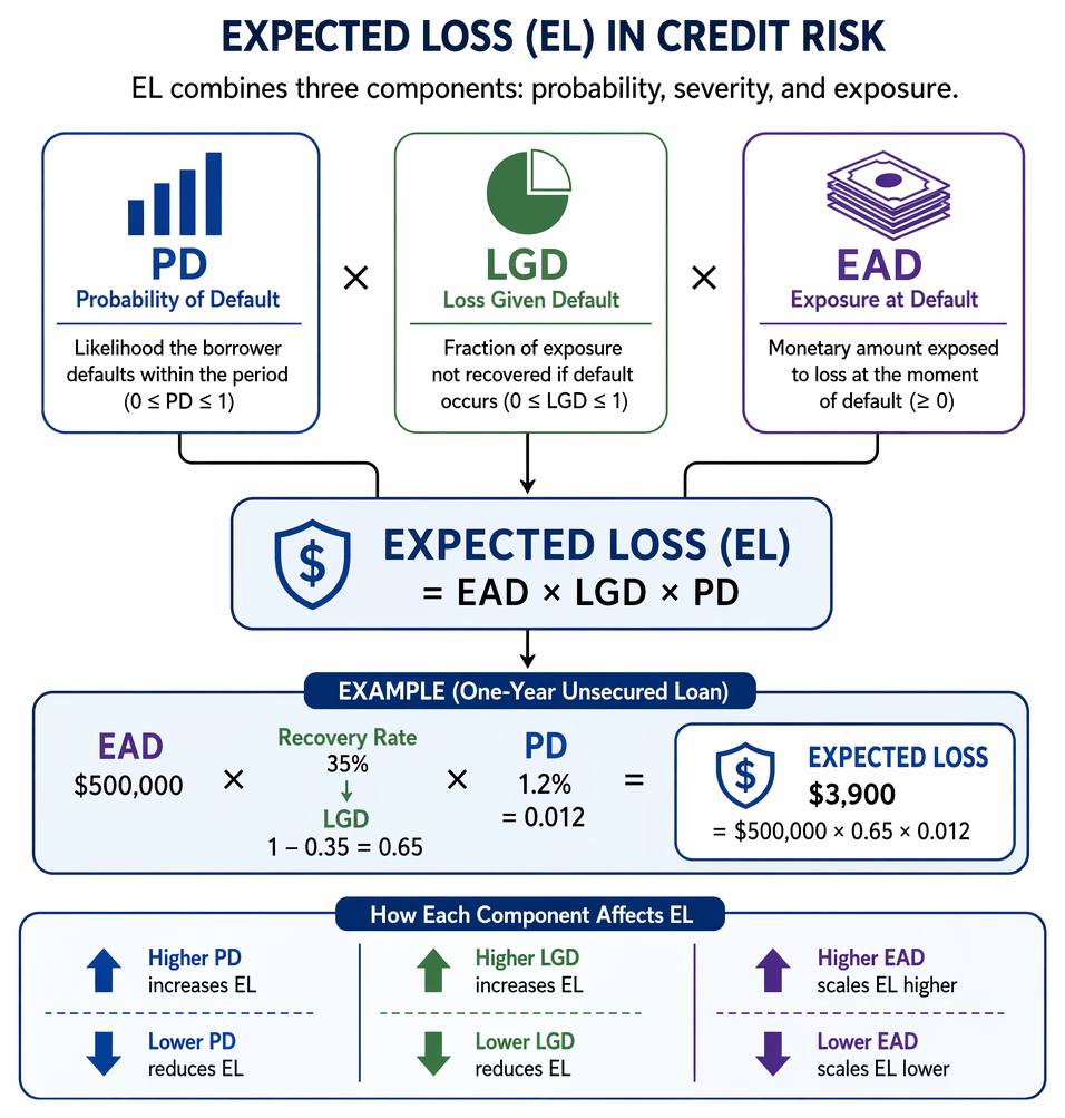
Credit risk reflects both the chance that a borrower will default and the extent of any resulting financial loss. The core formula for expected loss (EL) combines three elements:
Credit valuation adjustment is calculated by converting hazard rates into survival and marginal default probabilities, then discounting period expected losses.
- Probability of Default (PD): The likelihood of default during the period assessed.
- Loss Given Default (LGD): The fraction of exposure not recovered if default occurs.
- Exposure at Default (EAD): The monetary value exposed to loss at the moment of default.
For a single period (for example, one year), the expected loss is:
For loans and bonds over short horizons, EAD is often approximated by the current carrying value (for loans) or the risk-free present value of promised cash flows (for bonds). For revolving commitments, EAD includes current drawings plus an estimate of additional drawings at default. For derivatives, EAD is scenario-dependent and is usually approximated by expected positive exposure.
Worked Example 1.1
A bank holds a $500,000 unsecured loan to a company with a one-year probability of default of 1.2%. If the estimated recovery rate in the event of default is 35%, what is the expected loss?
Answer:
LGD =
Expected loss =
Expected loss = $3,900 The bank should treat $3,900 as the cost of expected credit losses over the year on this exposure.
Relationship between PD, LGD, and expected loss
Higher PD or higher LGD increase EL, while a higher recovery rate (lower LGD) reduces it. EAD scales the loss: doubling the exposure doubles EL if PD and LGD are unchanged.
From a portfolio strategy standpoint, a credit manager can reduce EL by:
- Reducing PD: improving underwriting standards, tightening covenants, or shifting toward higher-rated obligors.
- Reducing LGD: obtaining better collateral, improving seniority, or enhancing recovery processes.
- Reducing EAD: lowering individual exposure limits, shortening maturities, or reducing undrawn commitments.
Importantly, two exposures can have the same expected loss but very different risk profiles. For example, a high-PD/low-LGD position and a low-PD/high-LGD position can have similar EL, but the tail risk (unexpected loss) and capital needs differ. Level 2 questions may ask you to compare such profiles using EL and qualitative reasoning about recovery and concentration risk.
Multi-period expected loss, hazard rates, and survival
For horizons longer than one period, expected loss must incorporate:
- The conditional probability of default in each period (the hazard rate).
- The probability of survival up to each period.
- Potentially, time-varying EAD and LGD.
- Discounting of future expected losses to present value.
With a constant annual hazard rate , the survival probability to the end of year is:
The marginal probability of default in year is:
The expected loss in year is then:
and the present value of expected losses (CVA for a fixed-cash-flow instrument) is:
where are appropriate (risk-free) discount rates.
Recognizing the distinction between the hazard rate and the marginal PD is important. The hazard rate is typically specified per year, but the PD in later years declines relative to the hazard rate because fewer borrowers remain to default (some have already defaulted).
Worked Example 1.2
An analyst examines a $2 million portfolio of BBB-rated bonds. The one-year transition matrix gives a 4% probability of downgrade to BB (with an estimated 60% loss in market value upon downgrade relative to today’s value) and 1% probability of default (with LGD of 70% on the exposure). For simplicity, assume the bond’s price remains unchanged if the rating does not change. What is the expected loss due to these two outcomes in a year?
Answer:
- Loss from downgrade to BB = $2,000,000 × 0.04 × 0.60 = $48,000
- Loss from default = $2,000,000 × 0.01 × 0.70 = $14,000
- Total expected loss from transitions = $48,000 + $14,000 = $62,000
Note that here “LGD” for downgrade represents an estimated price decline on rating migration, whereas LGD for default represents unrecovered principal.
This example illustrates that credit migration, not just outright default, can drive expected losses via mark-to-market effects when a bond’s spread widens after downgrade.
CREDIT MIGRATION AND TRANSITION MATRICES
Borrowers’ credit quality may change over time. A credit migration matrix (or transition matrix) shows the probabilities of moving from one credit rating to another—including default—within a set period, typically one year.
A typical one-year transition matrix has:
- Rows: current rating (e.g., AAA, AA, A, BBB, BB, B, CCC).
- Columns: rating one year later, including a “Default” column.
- Each row summing to 1 (100%).
The diagonal entries (e.g., A→A) represent rating stability; off-diagonals represent migrations (upgrades and downgrades). The entry in the “Default” column for a given row is the one-year PD for that rating, but the matrix provides far richer information than a single PD.
Using a transition matrix, you can:
- Project the distribution of future ratings for a portfolio.
- Estimate multi-year default probabilities (by multiplying matrices, though in exam questions the relevant probabilities are usually given).
- Estimate expected mark-to-market losses by combining migration probabilities with current and future prices or spreads for each rating category.
In portfolio modeling, each future rating state is assigned a state value (price or spread). Expected price in one year is:
where is the transition probability to state and is the price if that state occurs.
APPLICATIONS TO CREDIT PORTFOLIO STRATEGIES
In credit portfolio management, expected loss (EL) serves as a basis for:
- Risk-based pricing: charging spreads that cover EL plus a premium for capital and profit.
- Loss forecasting and provisioning: setting aside reserves equal to portfolio EL over a given horizon.
- Capital allocation: allocating economic or regulatory capital to cover unexpected loss over EL at a target confidence level.
Portfolio strategies may include:
- Diversifying to manage exposure concentrations by obligor, sector, geography, and rating.
- Adjusting exposures to credits with changing transition (migration) probabilities, for example, trimming exposures to credits showing increased downgrade risk.
- Pricing facilities to cover EL and the cost of capital for unexpected loss.
- Using credit derivatives or insurance (such as credit default swaps) to transfer PD and/or LGD risk where justified by CVA and spread analysis.
- Managing the term structure of credit risk by comparing short- and long-maturity exposures using credit spread curves and term structures of PDs and LGDs.
A common application is comparing bonds using expected loss per $100 of par. The bond with the lowest expected loss has the lowest credit risk, other things equal; if it also offers a higher spread than its peers, it may be relatively attractive.
Worked Example 1.3
Three corporate bonds, each with $100 par, have the following characteristics for the next year:
- Bond X: exposure $102, recovery $40, PD 1.25%.
- Bond Y: exposure $88, recovery $45, PD 1.30%.
- Bond Z: exposure $92, recovery $32, PD 1.65%.
Which bond has the highest credit risk based on expected loss?
Answer:
First compute LGD (per $100 par) as exposure minus recovery. For X: LGD = $62, expected loss = = $0.775. For Y: LGD = $43, expected loss = = $0.559. For Z: LGD = $60, expected loss = = $0.99. Bond Z has the highest expected loss and therefore the highest credit risk on this metric. This example illustrates how expected loss blends PD and LGD; a bond with a slightly higher PD but much lower LGD could still be less risky.
CREDIT VALUATION ADJUSTMENT (CVA)
When valuing derivatives or other bilateral exposures, credit valuation adjustment (CVA) represents the present value of all expected credit losses due to the counterparty’s potential default.
Formally, for a given counterparty:
where:
- is expected exposure at time (risk-free valuation).
- is loss given default at time .
- is the marginal probability of default in period (hazard rate times survival from previous periods).
- is the discount rate (usually benchmark risk-free).
CVA can also be viewed as:
For fixed-cash-flow instruments (like a bond), expected exposure in each period is simply the risk-free present value of remaining promised cash flows at that future date. For derivatives, expected exposure depends on the distribution of relevant risk factors and is typically positive only when the instrument is in-the-money.
Key Term: Credit Valuation Adjustment (CVA)
CVA is the present value of expected credit losses on an instrument due to counterparty default; it equals the difference between its risk-free value and its value after accounting for counterparty credit risk.
Worked Example 1.4
A $10 million notional, five-year derivative contract has:
- Annual marginal PD (for simplicity) of 2%.
- Constant LGD of 55%.
- Annual expected positive exposure (EE) of $2 million.
- Flat risk-free discount rate of 0% (for simplicity).
Using simple annual periods and ignoring survival, the analyst initially estimates:
Annual expected loss = $22,000
What is (i) the total expected credit loss over 5 years under this simplification, and (ii) conceptually, how would a more precise calculation differ?
Answer:
Under the simplifying assumption, total expected loss = 5 × $22,000 = $110,000. A more precise calculation would:
- Use conditional marginal PDs (hazard rates) and survival probabilities so that PD in later years is applied only to the surviving exposure.
- Allow for time-varying EE and discount each year’s expected loss at risk-free rates. The correct CVA would therefore be slightly less than $110,000 because the same 2% hazard rate applied with survival implies marginal PDs below 2% in later years.
This illustrates that while simple EL approximations may ignore survival, exam problems that mention hazard rates or survival probabilities expect you to adjust marginal PDs appropriately.
Exam Warning: A frequent error is to omit compounding or not to adjust PD when using multi-year horizons. For multi-year periods, cumulative PD must reflect survival (i.e., non-default) up to each year. Always multiply period survival probabilities by hazard rates to obtain marginal PDs, and discount future expected losses to present value when computing CVA.
CREDIT MIGRATION, SPREADS, AND PRICE IMPACT
Credit ratings capture relative credit quality. A rating change affects a bond’s yield spread and price even if the issuer does not default. The Level 2 curriculum links rating migration to price changes via duration and spread changes.
When a bond’s rating changes, the change in price due to a change in credit spread can be approximated by:
where is measured in decimal form (e.g., 27 bps = 0.0027).
Worked Example 1.5
Suppose a bond with a modified duration of 6.32 is downgraded from AAA to AA. The typical AAA credit spread is 60 bps, while the typical AA credit spread is 87 bps. Assuming the bond is priced at typical spreads before the downgrade, estimate the percentage change in price due purely to the change in credit spread.
Answer:
\Delta \% P \approx -6.32 \times 0.0027 = -0.0171$$ or about a 1.71% price decline. This mark-to-market loss is a **migration loss**, not a default loss.
A credit migration matrix provides the probabilities of such downgrades (e.g., AAA→AA), while duration and spread data provide the severity in price terms. Together they allow you to compute expected migration losses.
POINT-IN-TIME PDs AND MIGRATION-BASED MODELING
Two broad approaches to default probability estimates appear in practice:
-
Point-in-Time (PIT) PDs:
- Estimated from current financial and macroeconomic data.
- Sensitive to the economic cycle (higher in recessions, lower in booms).
- Commonly used in regulatory expected-loss calculations and provisioning.
-
Migration-based (multi-state) modeling:
- Uses transition matrices to model movement among rating states (AAA, AA, ..., Default).
- PD is only one state (rating→default in one period); migration probabilities to other ratings are also modeled.
- Facilitates pricing and risk management that consider both default and non-default rating changes.
For the exam, be able to:
- Recognize that transition matrices model the entire rating process, not just default.
- Distinguish one-step PD (rating→default in one period) from cumulative PD over several periods, which must incorporate survival and repeated migrations.
Summary
Expected credit loss (EL) measures the average loss for a given exposure or portfolio and is essential for pricing, provisioning, and capital allocation. It combines three key components: PD (likelihood of default), LGD (loss severity given default), and EAD (amount at risk). Over multiple periods, EL is computed using hazard rates, survival probabilities, time-varying exposures, and discounting.
Credit migration matrices provide the probabilities required for predicting losses from rating downgrades and defaults. They are central to multi-state credit models that capture both default and migration risk. LGD quantifies the severity of loss upon default and depends on recovery rates, seniority, and collateral, while EAD reflects instrument-specific exposure profiles, including undrawn commitments and derivative exposures.
CVA extends the expected loss concept to derivatives and bilateral exposures by discounting expected credit losses over time, using expected exposure profiles, LGD, and marginal default probabilities. In portfolio strategies, these quantitative tools support diversification, concentration limits, risk-based pricing, and capital allocation, and they allow analysts to compare credit risk across instruments using expected loss and migration-driven price impacts.
Key Point Checklist
This article has covered the following key knowledge points:
- Expected loss for a single period equals .
- LGD is the percentage not recovered after default: .
- EAD reflects the amount at risk at default and differs across loans, revolving facilities, and derivatives.
- Hazard rates and survival probabilities are used to derive marginal and cumulative default probabilities over multiple periods.
- Credit migration (transition) matrices provide probabilities of rating upgrades, downgrades, and defaults, enabling estimation of expected migration and default losses.
- Rating downgrades cause mark-to-market losses, which can be approximated using modified duration and changes in credit spreads.
- CVA equals the present value of expected credit losses on an instrument and is the difference between its risk-free value and its risky value.
- Multi-period CVA calculations require marginal PDs (hazard rates), survival probabilities, expected exposures, LGD, and discounting.
- Portfolio strategies use PD, LGD, EAD, and migration information to set pricing, limits, and hedging strategies, and to allocate capital.
Key Terms and Concepts
- Expected Loss (EL)
- Loss Given Default (LGD)
- Recovery Rate
- Probability of Default (PD)
- Hazard Rate
- Probability of Survival
- Cumulative Probability of Default
- Marginal Probability of Default
- Exposure at Default (EAD)
- Expected Exposure
- Credit Migration (Transition) Matrix
- Point-in-Time Probability of Default
- Credit Spread
- Credit Valuation Adjustment (CVA)