Learning Outcomes
This article explains key aspects of futures and options overlays for portfolio risk management in the CFA Level 3 exam context, including:
- Using index and bond futures to adjust portfolio beta, duration, and asset‑class weights without disturbing underlying holdings.
- Distinguishing futures overlays from options overlays in terms of payoff profiles, downside protection, upside participation, and capital efficiency.
- Applying core formulas to size futures and options positions for beta and duration overlays, cash equitization, and tactical tilts.
- Interpreting exam‑style numerical examples involving equity index futures, protective puts, covered calls, collars, and duration overlays in liability‑relative settings.
- Evaluating implementation risks such as basis risk, contract expiry and roll yield, margin and liquidity demands, and governance or IPS constraints.
- Comparing derivatives overlays with physical rebalancing and other risk‑management tools, and identifying when overlays are the more efficient implementation choice.
- Integrating qualitative reasoning with calculations to write concise constructed‑response answers that link overlay recommendations to investor objectives, constraints, and business‑cycle views.
- Assessing the role of volatility derivatives and variance swaps alongside traditional option strategies as tail‑risk management overlays.
CFA Level 3 Syllabus
For the CFA Level 3 exam, you are required to understand the application of derivatives, specifically futures and options overlays, in the context of portfolio risk management, with a focus on the following syllabus points:
- Describe how futures contracts are used to manage or alter portfolio exposures.
- Explain how options overlays are constructed to control portfolio risk.
- Calculate and interpret the number of contracts needed for hedging and tactical overlays.
- Evaluate the risks and limitations associated with derivative overlays, including basis risk and transaction costs.
- Compare derivatives overlays with alternative risk management techniques.
- Demonstrate the use of derivatives in asset allocation, rebalancing, and equitizing cash.
- Discuss how derivatives can be used to align asset exposures with liability characteristics (e.g., duration matching).
- Demonstrate the use of volatility derivatives and variance swaps as tail‑risk overlays relative to more traditional option strategies.
- Interpret the interaction between business‑cycle expectations and tactical overlay decisions.
- Assess overlay strategies within the broader IPS and governance framework of institutional and private clients.
Test Your Knowledge
Attempt these questions before reading this article. If you find some difficult or cannot remember the answers, look more closely at that area during your revision.
-
What is the primary purpose of a futures overlay applied to an existing equity portfolio?
- a) To eliminate all unsystematic risk from the portfolio.
- b) To synthetically adjust market exposure (beta) without trading the existing securities.
- c) To increase stock-specific exposure using single-stock futures.
- d) To hedge currency risk arising from foreign holdings only.
-
How does an options collar overlay typically affect the risk–return profile of an equity portfolio?
- a) It removes all downside risk while keeping full upside potential.
- b) It increases both downside risk and upside potential by adding leverage.
- c) It limits downside risk below a floor and caps upside beyond a ceiling over the option’s life.
- d) It has no effect on the portfolio’s payoff pattern at expiry.
-
A manager oversees a fully invested $20 million equity portfolio with a beta of 1.0. The index future on the benchmark trades at 2,500, and each contract has a multiplier of $250. To fully hedge the market exposure using futures, the closest number of contracts is:
- a) Go short 20 contracts.
- b) Go short 32 contracts.
- c) Go short 80 contracts.
- d) Go long 32 contracts.
-
In the context of a futures overlay, what is “basis risk” most accurately?
- a) The risk that the futures position requires daily margining and creates liquidity risk.
- b) The risk that the futures price and the value of the hedged portfolio do not move in perfect lockstep.
- c) The risk that the futures contract expires before the manager can roll it.
- d) The risk that the exchange changes the contract multiplier during the hedge.
-
A portfolio is 40% in equities and 60% in bonds. The IPS allows a temporary equity range of 35%–45%. The manager becomes short‑term bullish and wants to move to an effective equity exposure of 50% for the next three months without selling bonds. Which implementation is most consistent with this objective and the overlay concept?
- a) Sell bonds and buy additional equities to reach 50% equity weight.
- b) Use an equity index futures overlay to add 10% notional equity exposure.
- c) Use a covered call strategy on the existing equities.
- d) Use protective puts on the existing equities.
-
A client holds a concentrated equity position that she is reluctant to sell because of large unrealized capital gains. She is very concerned about a 20% market correction over the next 6–12 months but still wants some upside participation. Which overlay is most appropriate?
- a) Short index futures equal to 100% of the position.
- b) Buy protective puts on the stock or an appropriate index.
- c) Sell uncovered calls on the stock.
- d) Invest surplus cash into additional equities.
-
A defined‑benefit pension plan has a duration gap: its asset BPV is significantly lower than its liability BPV. The sponsor wants to reduce surplus volatility without materially changing credit exposure. The most appropriate implementation is to:
- a) Extend the duration of the bond portfolio by buying longer‑maturity corporate bonds.
- b) Use Treasury bond futures overlays to increase asset BPV toward liability BPV.
- c) Increase equity exposure using equity index futures.
- d) Buy at‑the‑money equity index puts as a tail‑risk hedge.
-
A wealthy retiree’s IPS emphasises capital preservation over the next three years but acknowledges a strong aversion to paying large explicit option premia. Which overlay is most consistent with these preferences?
- a) A rolling program of deep in‑the‑money protective puts on 100% of the equity portfolio.
- b) A zero‑cost collar on a large portion of the equity portfolio, rolled annually.
- c) A leveraged long‑call position financed by borrowing against the portfolio.
- d) A systematic short‑put program on the equity benchmark.
Introduction
Derivative overlays using futures and options are essential portfolio management tools for risk and tactical exposure control at CFA Level 3. You are expected to identify situations where overlays are appropriate, perform calculations, and analyse key risks. Overlays enable managers to adjust or hedge systematic exposures efficiently—often to implement temporary tactical views, rebalance, or manage risk without disturbing existing portfolio holdings, which might be illiquid, tax-sensitive, or subject to client constraints.
Key Term: derivatives overlay
The use of exchange-traded or OTC derivative contracts, such as futures or options, layered on top of a physical asset portfolio to modify or hedge the portfolio’s risk exposures without changing the physical holdings.
Overlay management is particularly relevant for:
- Institutional portfolios rebalancing between asset classes (for example, using index futures instead of trading hundreds of individual securities).
- Private wealth portfolios where selling appreciated positions would trigger large capital gains taxes.
- Global multi-asset portfolios where tactical views change more frequently than the strategic asset allocation.
- Asset–liability portfolios (e.g., pension plans, insurers) needing to align asset duration or beta with liability characteristics without wholesale repositioning.
In the Level 3 curriculum, overlays sit at the intersection of risk management, asset allocation, and IPS implementation. Derivatives are not used in isolation; they are implementation tools for objectives stated elsewhere in the IPS:
- Reduce short-term downside risk without exiting long-term strategic positions.
- Maintain equity exposure during cash inflows/outflows to minimise tracking error.
- Temporarily tilt sector, region, or asset-class weights based on macro or business cycle views.
- Match the interest rate sensitivity of assets and liabilities in a surplus‑risk framework.
A critical exam skill is to connect the investor’s objectives and constraints in the IPS (e.g., aversion to realizing gains, desire to maintain strategic holdings, limits on leverage or derivatives) with the choice of overlay versus physical rebalancing. Derivative overlays are rarely an end in themselves; they are implementation tools for IPS-driven decisions.
Overlay programs are often run by specialist overlay managers who sit “on top” of multiple constituent portfolios. For example:
- A global equity manager runs regional sleeves.
- A separate overlay manager uses index futures on each region to keep total equity exposure within policy bands and to implement tactical tilts.
- An ALM committee for a pension fund sets a target surplus-risk profile; an overlay manager implements duration and equity-beta overlays to keep the plan close to that profile.
In a vignette, this type of governance structure often explains why the person making the futures or options decision is not the same as the primary stock-picker. You may be asked to comment on whether the overlay manager’s actions are consistent with the overall IPS, risk limits, or tactical bands.
Key Term: hedge ratio
The proportion of a specified exposure that is offset or modified with derivatives, often expressed as a fraction of market value or risk (e.g., beta, duration) that is hedged.
At Level 3 you must be comfortable thinking in terms of hedge ratios, not just “all‑or‑nothing” hedges. For instance, a manager might hedge only 50% of equity beta or 70% of duration to reflect views, constraints, or tolerance for basis risk. Essay questions often test whether you can justify a partial hedge quantitatively and qualitatively:
- Show the formula and compute the number of contracts; and
- Explain why the hedge is partial (e.g., maintain some upside, avoid over‑hedging due to basis risk, respect derivatives‑usage limits).
Key Term: tracking error
The standard deviation of the active return of a portfolio relative to its benchmark; in overlay contexts, it is the variability in performance caused by overlays not perfectly matching benchmark moves.
Because many overlay programs exist primarily to keep tracking error within a desired range (for example, equitizing cash in an index fund), you should be able to explain how futures and options overlays affect tracking error relative to the benchmark:
- Cash drag and under‑investment increase tracking error.
- A well‑sized futures overlay reduces tracking error (by replicating benchmark beta).
- Aggressive tactical overlays may increase tracking error by design.
There is also a strong link to macro and business cycle analysis. Tactical overlays are often motivated by views about the phase of the cycle (e.g., early expansion vs slowdown), but the curriculum emphasises that such forecasts are noisy. Historical evidence shows large variation in the length and intensity of expansions and recessions, and markets can anticipate turning points well before they show up in macro data. This is why many overlays are sized conservatively and constrained by IPS tactical bands, and why exam answers should acknowledge the uncertainty associated with business-cycle timing.
For example:
- In an initial recovery or early expansion, a committee may authorise a temporary beta increase using equity index futures, expecting improving growth and supportive policy.
- In a slowdown or late expansion, they might reduce beta or shorten duration using overlays, anticipating tighter policy and rising yields.
- In a contraction, overlays might be used to add duration or implement downside equity protection, even while the strategic allocation remains unchanged.
A high‑quality Level 3 answer will recognise that such macro‑driven overlays should be implemented with awareness of their risk: mis‑timing the cycle can create negative active returns and raise tracking error. You are expected to comment not only on what overlay to use but also on how confidently and for how long to apply it, given the noisy signal from business‑cycle indicators.
Test Tip: When revising Futures and options overlays, connect each definition, method, or rule to the kind of question the assessment is likely to ask.
Exam Warning: Do not rely on keyword recognition alone; check the precise condition, exception, calculation step, or evidence the question requires.
Business‑cycle phases and overlay choices
The business‑cycle reading decomposes expansions and recessions into five phases with characteristic capital‑market behaviour. Understanding these patterns helps you justify overlay recommendations:
-
Initial recovery (just after the trough):
- Macroeconomy: Growth picks up from a low base, policy is still highly stimulative, inflation is decelerating, and the output gap is large.
- Markets: Short‑term rates are very low, longer‑term yields are bottoming, and equities—especially cyclical and high‑beta assets—often rally strongly.
- Overlay implications: It can be reasonable to use equity index futures to raise portfolio beta or to equitize cash quickly, as the opportunity cost of being underweight risk assets is high. Duration‑reduction overlays are usually premature at this stage; if anything, a modest long‑duration overlay may still be justified.
-
Early expansion:
- Macroeconomy: Growth broadens, unemployment begins to fall, housing and consumer durables strengthen, and profits rise rapidly.
- Markets: Central banks start to remove stimulus, short rates rise, the yield curve flattens gradually, and equities generally trend upward.
- Overlay implications: Overweighting equities with futures can still be justified but should be sized more conservatively. Managers might also begin to reduce excess duration via bond‑futures overlays if inflation risks are building.
-
Late expansion:
- Macroeconomy: The output gap closes, inflation and wages rise, capacity constraints appear, and central banks turn restrictive.
- Markets: Short rates and bond yields generally rise, the curve flattens further, and equity markets may climb but with increased volatility.
- Overlay implications: This phase often calls for reducing equity beta using short index futures and shortening duration using bond‑futures overlays. Tail‑risk hedges with options may be appropriate as the risk of an adverse shock increases.
-
Slowdown:
- Macroeconomy: Growth decelerates, investment projects become less attractive, and accumulated debt burdens weigh on activity.
- Markets: Short rates are high but near their peak, government bond yields may top out and then fall, the curve can invert, and credit spreads widen. Equities often perform poorly, with quality and defensive sectors outperforming.
- Overlay implications: Equity managers may implement partial or full beta‑reduction overlays; fixed‑income managers often start adding duration with futures to benefit from falling yields. Option‑based downside protection becomes more attractive, but implied volatility is often elevated, raising the cost.
-
Contraction (recession):
- Macroeconomy: Output and profits fall, unemployment rises, and default risks increase. Policy is eased aggressively once the downturn is recognised.
- Markets: Short and long rates decline, the yield curve steepens, equities typically sell off early in the phase and then bottom before the economy, and credit spreads remain wide until recovery expectations improve.
- Overlay implications: Long bond‑futures overlays to increase duration can both stabilise surplus for institutions and add return. On equities, managers may choose between maintaining hedges (if they expect further weakness) and gradually removing beta hedges to participate in an eventual recovery.
The reading also stresses that these patterns are averages; actual cycles differ widely in duration and intensity. For exam purposes, when you link an overlay decision to a business‑cycle phase, explicitly acknowledge this uncertainty (“signals are noisy,” “phases vary in length”) and recommend position sizes that are credible within IPS tactical bands rather than extreme all‑in bets.
Key Term: tail‑risk hedge
A derivative overlay, typically using deep out‑of‑the‑money puts or long volatility positions, designed primarily to protect the portfolio against large, infrequent adverse market moves rather than routine volatility.
The rest of this article distinguishes between futures overlays and options overlays, develops the key formulas, and places them in realistic Level 3-style contexts, including asset allocation shifts and liability-relative objectives.
Futures Overlays
A futures overlay allows quick, efficient changes to a portfolio’s asset allocation or risk profile. This is accomplished by adding or reducing notional exposure using liquid exchange-traded futures contracts tied to market indexes or interest rates.
Key Term: futures overlay
The process of buying or selling futures contracts to increase or decrease portfolio exposure to a specific market or risk factor without trading the actual securities. Key Term: contract multiplier
A fixed amount by which the quoted futures price is multiplied to obtain the notional value of one futures contract (for example, $250 per index point for some equity index futures). Key Term: beta overlay
The use of derivatives, typically equity index futures, to raise or lower the overall beta (systematic risk) of a portfolio relative to a benchmark without changing the actual securities.
Why use futures rather than cash securities
Relative to trading the cash securities, index futures typically offer:
- Speed of execution, especially when changing exposure to an entire market or sector.
- Low explicit transaction costs per unit of notional exposure.
- Capital efficiency, because only margin is posted while remaining capital stays invested.
- Ease of reversing the position if views change.
- Ability to implement exposures in markets that may be difficult to access directly (for example, foreign equity markets with capital controls).
Capital efficiency is not just a buzzword. Futures exchanges generally require initial margin of roughly 3%–15% of notional value (depending on underlying volatility), whereas financing a similar exposure with cash equities could require tying up 100% of capital or using margin borrowing that increases balance‑sheet leverage. With futures, the bulk of the portfolio can continue to earn returns in its existing investments while the overlay fine‑tunes risk exposures. For institutional accounts, this is a central reason to prefer futures for short‑term tilts.
These advantages explain why futures overlays feature heavily in exam questions dealing with tactical asset allocation and short‑term risk management. In many vignettes the portfolio is large and diversified, and the text explicitly flags high transaction costs or tax costs on physical trades—strong hints that a futures overlay is preferred.
Key Term: cash equitization
A strategy that uses derivatives (typically equity index futures) to provide equity-like exposure on cash holdings so that the overall portfolio tracks an equity benchmark more closely.
When you see “excess cash,” “uninvested cash,” or “delays in funding” in a vignette about an equity index fund, you should immediately think of cash equitization using equity index futures. The objective is not to outperform the benchmark but to avoid unintentional under‑investment.
Beyond index funds, similar logic applies for:
- Transition management (between managers or benchmarks).
- Temporary defensive positions where the manager sells some physical equities but wants the option to quickly re‑enter using futures.
- Multi‑currency portfolios, where local markets are illiquid but index futures in a major financial centre (e.g., Chicago, Eurex) are deep and cheaper to trade.
In your exam reasoning, you should explicitly contrast these implementation advantages with any disadvantages mentioned in the vignette, such as leverage constraints or governance concerns about derivatives.
Typical Uses
- Equity exposure adjustment: Increase or decrease equity beta swiftly without trading the cash equities.
- Tactical asset allocation: Temporarily tilt exposure to asset classes, sectors, or regions (e.g., overweight German equities, underweight Italian equities).
- Implementing rebalancing: Return to policy targets efficiently when markets move away from strategic weights, especially when portfolios hold many illiquid securities.
- Temporary cash equitization: Maintain market exposure while holding cash to minimize tracking error to an equity benchmark.
- Interest rate and duration management: Adjust portfolio duration using government bond futures as an overlay on top of existing bond holdings.
- Cross-hedging: Use futures on a broad index to hedge a portfolio that is correlated with, but not identical to, the index (introducing basis risk).
- Separating alpha from beta: Neutralize market exposure (beta) of an active equity portfolio with stock index futures, leaving only stock-selection alpha.
- Transition management: Maintain continuous market exposure when changing external managers or transitioning between benchmarks (e.g., old index to new index).
In a constructed‑response question, after identifying the appropriate overlay, you should explicitly tie the use case to the IPS:
- Is the goal risk reduction, tactical tilting, or benchmark tracking?
- Is the overlay temporary (tactical) or long‑term (structural)?
- Does the use of futures respect derivatives and leverage constraints?
You may also be asked to evaluate whether derivatives should be used at all. For example:
- A strategic change in equity allocation from 40% to 60% over the next five years is better implemented through gradual physical rebalancing, not a permanent futures overlay.
- A short‑term desire to overweight equities for the next quarter is well suited to a futures overlay, with clear plans for when to unwind the position.
Recognising the horizon of the view relative to the life of the derivative contract, and relative to the strategic horizon in the IPS, is an important evaluative skill.
Mechanics: Long vs Short Futures
Recall the basic directional exposures:
- Long equity index futures: gain when the index rises, lose when it falls → increase equity exposure.
- Short equity index futures: lose when the index rises, gain when it falls → decrease equity exposure.
- Long bond futures: benefit from falling yields (rising bond prices) → effectively increase duration.
- Short bond futures: benefit from rising yields (falling bond prices) → effectively decrease duration.
Margin requirements introduce leverage: a relatively small cash outlay (initial margin) controls a large notional exposure. This leverage magnifies both desired and undesired outcomes, so margin and liquidity considerations must always be mentioned in exam answers. If the IPS limits leverage or derivatives use, you should explain whether the proposed overlay is permissible.
It is also worth distinguishing briefly between forwards and futures in overlay contexts:
- Forwards are OTC, customizable, and expose the investor to counterparty risk plus lower liquidity.
- Futures are exchange‑traded, standardized, centrally cleared, and typically preferred for overlay programs due to liquidity and operational ease.
Level 3 questions focused on overlays almost always use futures, but you may be asked why futures are chosen instead of forwards or swaps. A common justification is that futures provide efficient, transparent exposure with low counterparty risk, which fits the governance and regulatory requirements of many institutional investors.
Worked Example 1.1
A manager wants to add $10 million equity exposure for 10 days using S&P 500 futures while a cash inflow settles. Each S&P 500 future contract is valued at $200,000. How many contracts should the manager buy?
Answer:
The required number of contracts is
The manager should go long 50 S&P 500 futures contracts to replicate the required exposure until receiving the cash. This is an example of cash equitization. In a written response you should add that:
- The overlay keeps the effective equity weight close to the policy target, reducing unintended tracking error versus the equity benchmark.
- The exposure is temporary and easily reversed by closing the futures when the cash is invested.
- The manager must ensure sufficient liquid assets to meet potential variation margin calls if the market moves against the futures position during those 10 days.
- The overlay keeps the effective equity weight close to the policy target, reducing unintended tracking error versus the equity benchmark.
- The exposure is temporary and easily reversed by closing the futures when the cash is invested.
- The manager must ensure sufficient liquid assets to meet potential variation margin calls if the market moves against the futures position during those 10 days.
Calculating Hedge Ratios: Simple Notional Overlay
For a simple exposure change using futures, the standard formula for the number of contracts required is:
= \frac{\text{Desired exposure change}}{\text{Futures contract value}} = \frac{\Delta S}{F_0 \times \text{multiplier}}$$ where: - $\Delta S$ = desired change in dollar exposure to the asset class - $F_0$ = current futures price (index level or bond price) - $\text{multiplier}$ = contract multiplier (e.g., $250$ per index point) This is appropriate when: - The portfolio closely resembles the futures reference index (same index, beta near 1). - The objective is to add or remove a specific dollar amount of exposure (e.g., equitize \$20 million of cash, reduce exposure to Italian equities by €100 million). - We are not explicitly changing the portfolio’s beta; we are only adding or subtracting notional exposure in the same risk profile. In exam questions, always: - Convert the quoted futures price into contract value by multiplying by the contract multiplier. - State clearly whether the result implies buying (positive number) or selling (negative number) contracts. - Comment on whether the overlay respects IPS tactical bands and constraints (e.g., maximum equity weight, maximum synthetic exposure). You will often need to round the contract number to an integer. You should then: - State the rounded number. - Briefly comment that this introduces a small mismatch (as in the reading’s example where 44.44 contracts are rounded to 44), but that the residual exposure is typically negligible. For more complex hedges—for example, hedging a portfolio of small‑cap stocks with a broad‑market future—the optimal hedge ratio would theoretically incorporate the correlation and relative volatility between the portfolio and the futures index. In practice, Level 3 questions either give you a specific formula or stay with the simpler notional or beta‑based approaches discussed here. ### Calculating Hedge Ratios: Changing Portfolio Beta For risk‑factor overlays (e.g., reducing or increasing portfolio beta), you must account for the beta of both the portfolio and the futures contract. The standard CFA formula is: $$N_f = \left( \frac{\beta_T - \beta_S}{\beta_f} \right) \left( \frac{S}{F_0 \times \text{multiplier}} \right)$$ where: - $N_f$ = number of futures contracts (positive = buy, negative = sell) - $\beta_T$ = target portfolio beta - $\beta_S$ = current portfolio beta - $\beta_f$ = beta of the futures contract (typically ≈ 1 for broad index futures) - $S$ = current market value of the equity portfolio - $F_0 \times \text{multiplier}$ = contract value Interpretation: - If $\beta_T \< \beta_S$ (want to reduce risk), $N_f$ will be negative: sell futures. - If $\beta_T > \beta_S$ (want to increase risk), $N_f$ will be positive: buy futures. - For a full market hedge, set $\beta_T = 0$; the formula simplifies to: $$ N_f = - \left( \frac{\beta_S}{\beta_f} \right) \left( \frac{S}{F_0 \times \text{multiplier}} \right)$$ This beta‑based hedge ratio is more robust than a simple notional hedge whenever the portfolio’s beta differs materially from 1 or when the futures index differs from the benchmark in the IPS. In a constructed‑response answer you should explain why you are using the beta‑based formula and what assumptions it embeds: - Beta is estimated reasonably accurately and stays stable over the hedge horizon. - The portfolio’s return is highly correlated with the futures index. - Non‑market exposures (style, sector, small‑cap tilts) are not being hedged. You are also expected to interpret the economic meaning of the hedge ratio, not just compute it mechanically. A good answer will often relate the resulting effective beta to the manager’s macro view and risk budget. ### Worked Example 1.2 A defensive equity portfolio is worth £40 million with $\beta_S = 0.85$. The manager wants to increase the portfolio beta to $\beta_T = 1.10$ for the next three months using FTSE 100 index futures. The futures price is 7,300, the contract multiplier is £10, so each contract is worth £73,000. The futures beta is $\beta_f = 1.0$. How many FTSE 100 futures should be traded, and in which direction? > **Answer:** > Apply the beta overlay formula: > > $$> N_f = \left( \frac{1.10 - 0.85}{1.0} \right) > \left( \frac{£40{,}000{,}000}{£73{,}000} \right) > = 0.25 \times 547.95 \approx 137$$ > > $$> N_f$$ > > is positive, so the manager should buy 137 FTSE 100 futures. This raises the combined stock‑plus‑futures beta to approximately 1.10. > To demonstrate understanding in an essay, you could: > **Show that if the market rises 2%, the expected portfolio return is approximately:** > > $$> 1.10 \times 2\% = 2.2\%$$ > > **Verify with numbers: the stock portfolio return is:** > > $$> 0.85 \times 2\% = 1.7\%$$ > > The overlay via futures supplies the extra 0.5 percentage points. > **Explain that the tactical view is short term; hence futures are preferred to physically replacing defensive stocks with higher‑beta stocks, which would incur transaction costs and potentially disrupt the manager’s long‑term stock‑selection process.** > **Show that if the market rises 2%, the expected portfolio return is approximately:** > > $$> 1.10 \times 2\% = 2.2\%$$ > > **Verify with numbers: the stock portfolio return is:** > > $$> 0.85 \times 2\% = 1.7\%$$ > > The overlay via futures supplies the extra 0.5 percentage points. > **Explain that the tactical view is short term; hence futures are preferred to physically replacing defensive stocks with higher‑beta stocks, which would incur transaction costs and potentially disrupt the manager’s long‑term stock‑selection process.** ### Worked Example 1.3 A \$120 million equity portfolio has $\beta_S = 1.20$. The CIO wants to reduce the effective beta to $\beta_T = 0.60$ for the next month due to an expected market correction but does not want to sell stocks for tax reasons. The index future on the benchmark trades at 3,000 with a contract multiplier of \$250, and $\beta_f = 1.0$. How many futures should be used, and in what direction? > **Answer:** > Use the beta overlay formula: > > $$> N_f = \left( \frac{0.60 - 1.20}{1.0} \right) > \left( \frac{120{,}000{,}000}{3{,}000 \times 250} \right) > = (-0.60) \times \frac{120{,}000{,}000}{750{,}000} > = (-0.60) \times 160 = -96$$ > > The manager should sell 96 futures contracts. This overlay halves the portfolio’s market sensitivity without realizing capital gains on the existing stocks. Residual risk remains due to basis risk and estimation error in beta. > The decision to hedge only to > > $$> \beta_T = 0.60$$ > > rather than to zero reflects a partial hedge. You should justify this by noting that: > > - The CIO still wants some equity participation if the correction is milder than feared. > - Over‑hedging could lead to significant underperformance if markets rise. > - The IPS may restrict large directional bets, so completely eliminating equity beta might violate risk‑budget or tracking‑error guidelines. > - The CIO still wants some equity participation if the correction is milder than feared. > - Over‑hedging could lead to significant underperformance if markets rise. > - The IPS may restrict large directional bets, so completely eliminating equity beta might violate risk‑budget or tracking‑error guidelines. ### Futures Overlays for Duration Management Interest rate risk for bond portfolios can be overlaid using government bond futures. Conceptually this is parallel to beta management in equities, but the relevant risk measure is duration or basis point value (BPV) rather than beta. > **Key Term: duration overlay** > The use of interest rate derivatives (typically government bond futures or interest rate swaps) to increase or decrease the effective duration of a bond portfolio without trading the existing bonds. > **Key Term: basis point value (BPV)** > The change in the price (or present value) of a bond or portfolio for a 1 basis point (0.01%) change in yield, usually expressed in currency units. Rules of thumb: - To increase portfolio duration: go long bond futures. - To decrease duration: go short bond futures. The hedge is often expressed in terms of BPV: $$N_f = \frac{BPV_T - BPV_P}{BPV_{\text{CTD}}} \times \text{conversion factor}$$ where: - $BPV_T$ = target BPV for the portfolio (desired interest rate sensitivity) - $BPV_P$ = current BPV of the portfolio - $BPV_{\text{CTD}}$ = BPV of the cheapest‑to‑deliver bond into the futures, per contract - conversion factor = futures contract’s conversion factor (adjusts the CTD to the contract standard) > **Key Term: cheapest to deliver (CTD)** > The specific bond in the deliverable basket for a bond futures contract that is least costly for the short futures position to deliver, after adjusting for the contract’s conversion factor. An equivalent formulation sometimes used is based on dollar duration ($DD$): - $DD = \text{modified duration} \times \text{value}$ - $N_f = (DD_T - DD_P)/DD_f$, where $DD_f$ is the dollar duration of one futures contract (often derived from the CTD and conversion factor). You are unlikely to be asked to derive these formulas, but you may need to apply them and explain why a manager uses bond futures to align asset duration with liability duration in a liability‑relative context. In such questions, remember that the target BPV is typically the liability BPV or a policy benchmark BPV, consistent with surplus optimisation and hedging/return‑seeking concepts in the institutional asset allocation readings. In practice there are two layers of judgement: - How much of the liability interest‑rate risk to hedge (full vs partial BPV match). - Whether the hedge is implemented with futures, swaps, or physical bonds. Swaps may be preferable for long‑dated, customised hedges, whereas exchange‑traded bond futures are often chosen for shorter‑horizon tactical overlays or where liquidity and daily marking‑to‑market are important. ### Worked Example 1.4 A defined‑benefit pension fund holds a \$200 million bond portfolio with $BPV_P$ = \$90,000. The plan's liabilities have $BPV_L$ = \$135,000, and the CIO wants to match asset and liability BPV using Treasury bond futures. Each futures contract's CTD has $BPV_{\text{CTD}}$ = \$75 and a conversion factor of 1.05. How many futures contracts are required, and in which direction? > **Answer:** > The target BPV for the portfolio is the liability BPV: > > $$> BPV_T = 135{,}000$$ > > The required change in BPV is: > > $$> BPV_T - BPV_P = 135{,}000 - 90{,}000 = 45{,}000$$ > > Use the BPV hedge formula: > > $$> N_f = \frac{45{,}000}{75} \times 1.05 = 600 \times 1.05 = 630$$ > > Because the target BPV is higher than the current BPV, the manager must go long 630 futures contracts to increase duration. > A strong Level 3 explanation would note that: > > - Increasing asset BPV towards liability BPV reduces surplus volatility to parallel shifts in the yield curve. > - The fund is effectively increasing its sensitivity to falling yields (which increase both asset and liability values) so that the net surplus is more stable. > - Duration matching via futures leaves the underlying credit exposures and issuer mix unchanged, which is often desirable when liabilities are largely interest‑rate driven. > - Increasing asset BPV towards liability BPV reduces surplus volatility to parallel shifts in the yield curve. > - The fund is effectively increasing its sensitivity to falling yields (which increase both asset and liability values) so that the net surplus is more stable. > - Duration matching via futures leaves the underlying credit exposures and issuer mix unchanged, which is often desirable when liabilities are largely interest‑rate driven. ### Duration Overlays in a Hedging/Return‑Seeking Framework The asset–liability readings introduce approaches such as surplus optimization and the hedging/return‑seeking (two‑portfolio) framework. Duration overlays fit naturally into these frameworks. > **Key Term: surplus optimization** > A liability‑relative asset‑allocation approach that applies mean–variance optimization to surplus returns, using surplus volatility (asset return minus liability return) as the key risk measure instead of asset volatility alone. > **Key Term: hedging/return‑seeking portfolios approach** > A liability‑relative framework that separates assets into a liability‑hedging portfolio designed to match the characteristics of liabilities, and a return‑seeking portfolio aimed at generating surplus growth. In a surplus optimization context: - The objective function trades off expected surplus return against surplus volatility. - The “surplus efficient frontier” shows combinations of asset classes that optimise this trade‑off. - Implementing a duration overlay can move the plan along this frontier—reducing surplus volatility for a given asset mix—without costly reallocation among asset classes. Example: A pension plan invested partly in long corporate bonds and partly in equities may find that its surplus efficient frontier suggests slightly longer duration than that of its current bond allocation. Instead of selling and buying bonds, it can: - Keep its existing credit and alternative allocations unchanged. - Use long Treasury bond futures to add incremental BPV and bring total asset BPV closer to that implied by the surplus‑optimal portfolio. In the hedging/return‑seeking framework: - The hedging portfolio holds assets chosen to mimic liability sensitivities, notably interest‑rate exposure. - The return‑seeking portfolio holds higher‑return assets such as equities, private equity, and real estate. - A duration overlay is applied primarily to the hedging portfolio to fine‑tune the BPV match to liabilities. For instance, with a positive funding surplus, an ALM committee might: - Allocate enough assets to the hedging portfolio such that its BPV matches a high percentage (e.g., 90%) of liability BPV, using a combination of long bonds and futures. - Allocate the remaining surplus to return‑seeking assets that are unconstrained by liability duration, possibly hedging their equity beta using index futures when risk budgets are tight. A well‑reasoned exam answer distinguishes clearly between: - Duration overlays used as **hedging tools** to control surplus volatility, and - Equity futures overlays used in the **return‑seeking portfolio** to adjust beta. ### Futures in Tactical Asset Allocation and Rebalancing Relative to physical trading, futures overlays allow: - Fast implementation: You can change exposures intraday rather than trading many constituent securities. - Capital efficiency: Only margin is posted; the remainder of capital can remain invested in alpha‑generating strategies. - Reversibility: Tactical views can be reversed by closing or rolling futures contracts. - Precision: Exposures can be adjusted in relatively fine increments (e.g., add exactly €50 million of German equity exposure). In an exam vignette, if the question describes: - A temporary tactical view (“bearish on eurozone equities for the next quarter”), or - A desire to avoid transaction costs and taxes on existing securities, a futures overlay is usually the preferred implementation tool. > **Key Term: hedge ratio** > (revisited) > In this context, the hedge ratio links the notional value of futures to the exposure being adjusted (e.g., “hedge 30% of equity exposure” or “add €50 million to German equities”). You should always be able to move between the verbal description of the hedge and the corresponding contract count. A typical Level 3 question may give you multiple ways to implement the same view: - Sell $X$ of Italian equities and buy $X$ of German equities. - Use FTSE MIB and DAX futures to adjust exposures. - Do nothing and remain at policy weights. You should recommend the futures overlay when: - The view is short term relative to the strategic horizon. - The IPS highlights high trading costs or tax concerns. - Derivatives use is explicitly allowed. You should also relate tactical overlays to business‑cycle expectations: - In a late‑expansion phase with rising rates and tight credit, a manager might reduce cyclical equity exposure via index futures, while leaving long‑term holdings intact. - In an initial recovery, the same manager might temporarily overweight equities or credit using futures, anticipating that being underweight risk assets at that stage has a high opportunity cost. The curriculum stresses that such macro signals are noisy; therefore, tactical overlays are often constrained to modest deviations from policy (for example, ±5% around strategic equity weights) and are sized using risk‑budget metrics such as tracking‑error limits. ### Worked Example 1.5 A €500 million balanced fund is currently 60% equities and 40% bonds. The IPS strategic allocation is 55% equities and 45% bonds, with ±5% tactical bands. After a rally in equities, the manager wants to temporarily move to 65% effective equity exposure (bullish view) for the next three months without selling bonds. The equity benchmark future (beta 1.0) trades at 2,500 with a €10 multiplier. How many futures contracts should be bought? > **Answer:** > Current equity exposure is: > > $$> 0.60 \times 500 = €300$$ > > million. > Target effective equity exposure is: > > $$> 0.65 \times 500 = €325$$ > > million. > Desired increase in equity exposure is therefore: > > $$> \Delta S = 25$$ > > million. > Contract value is > > $$> F_0 \times \text{multiplier} = 2{,}500 \times 10 = €25{,}000$$ > > Number of contracts: > > $$> N_f = \frac{\Delta S}{F_0 \times \text{multiplier}} > = \frac{25{,}000{,}000}{25{,}000} > = 1{,}000$$ > > The manager should buy 1,000 equity index futures to increase effective equity exposure to 65% while leaving the physical 60/40 holdings unchanged. This is a classic tactical asset allocation overlay. > In a constructed‑response answer, you would also: > > - State that 65% is at the top of the permitted tactical band (55% ± 10%), so the overlay is IPS‑compliant. > - Emphasise that because the bullish view is explicitly short term, using futures avoids unnecessary turnover in the bond portfolio. > - Mention that if the bullish view proves wrong, the overlay can be quickly unwound, limiting further downside. > - State that 65% is at the top of the permitted tactical band (55% ± 10%), so the overlay is IPS‑compliant. > - Emphasise that because the bullish view is explicitly short term, using futures avoids unnecessary turnover in the bond portfolio. > - Mention that if the bullish view proves wrong, the overlay can be quickly unwound, limiting further downside. For more complex situations with multiple regional or sector tilts, the logic is the same, but you may have to size separate futures positions for each index involved (e.g., sell FTSE MIB futures to reduce Italian equity exposure and buy DAX futures to increase German exposure), as illustrated in the curriculum’s Rossi example. In such cases, a clear table of “current vs desired exposures” followed by contract calculations for each leg is a good way to structure your answer. ### Cash Equitization and Synthetic Indexing Cash holdings arise for many reasons: recent contributions, pending withdrawals, portfolio transitions, or anticipation of tactical moves. If the benchmark is an equity index, cash drag will cause underperformance unless the manager provides synthetic equity exposure. The futures-based cash equitization formula is a special case of the beta overlay formula where the cash has $\beta_S = 0$ and the target beta is 1.0 (or the benchmark beta): $$N_f = \left(\frac{\beta_T}{\beta_f}\right)\left(\frac{S}{F_0 \times \text{multiplier}}\right)$$ This is essentially the same formula used in the swaps/futures reading for “synthetic index” strategies. Key points to emphasise: - The objective is to minimise tracking error, not to take an active view. - The overlay should be sized for the cash amount, not the entire portfolio. - The cash remains in money market or short‑term instruments; the futures provide the beta exposure. The swaps reading notes that synthetic indexing can also be achieved by combining options (long call and short put at the same strike) instead of using futures. This structure replicates the payoff of a long forward and hence of the underlying index. In practice, however, futures are more common for equitization because: - They are usually more liquid than longer‑dated at‑the‑money options. - There is no explicit premium outlay (only margin). - Transaction costs for rolling are typically lower than for rolling a call/put combination. Exam pitfalls include: - Forgetting to multiply the futures price by the contract multiplier. - Hedging the entire portfolio instead of only the unintended cash portion. - Ignoring the beta of the futures contract when it differs from 1. Being explicit about these points in your answer can distinguish it from a purely mechanical calculation. ### Term Structure, Roll Yield, Contango, and Backwardation Futures overlays must typically be maintained over time by “rolling” positions from a near‑maturity contract into a later contract. This introduces additional considerations. > **Key Term: contango** > A futures term structure in which longer‑dated futures prices are higher than near‑dated futures prices or the expected future spot price. > **Key Term: backwardation** > A futures term structure in which longer‑dated futures prices are lower than near‑dated futures prices or the expected future spot price. > **Key Term: roll yield** > The return component arising from the convergence of a futures price toward spot as maturity approaches, positive in backwardation and negative in contango for a long futures position. When rolling a long futures overlay: - In backwardation, the manager sells the expiring contract at a higher price and buys the longer‑dated one at a lower price, generating positive roll yield. - In contango, the manager’s roll yield is negative: the new contract is more expensive, so maintaining the overlay has an ongoing cost. For equity index futures, contango or backwardation is usually modest and driven by interest rates and dividends, so roll yield is often small. For volatility futures (discussed later) or some commodity futures, term structure effects are much more significant and must be explicitly considered in overlay design. In an exam, if you are asked about the ongoing cost of a long futures overlay, you should discuss: - The financing component (interest rate minus dividend yield). - The roll yield (contango/backwardation). - Transaction costs around each roll date. And you should recognise that roll risk is part of implementation risk, not market direction risk: even if your view on the underlying index is correct, an adverse term structure can erode overlay performance. ### Practical Implementation Details for Futures Overlays In written answers, beyond the contract calculations you should address: - Margin and liquidity: Does the portfolio have sufficient liquid assets to meet potential variation margin calls if markets move against the overlay? - Alignment with IPS: Are derivatives permitted? Is leverage allowed? Are there regulatory constraints (e.g., for UCITS or insurance portfolios)? - Operational capacity: Does the manager have the systems to monitor futures positions, margin, and basis risk daily? - Measurement of success: Is the goal to reduce overall volatility, reduce tracking error, or match liability sensitivities? How will that be monitored (e.g., surplus risk metrics for pensions)? You may also be asked to comment on which contract to use when multiple maturities are available. Qualitatively: - Short‑dated contracts minimise basis risk relative to spot and are often more liquid. - Longer‑dated contracts reduce the frequency of rolls but may be less liquid and involve greater term‑structure risk. Your recommendation should reflect the horizon of the overlay: a hedge for the next two months typically uses the near‑month contract; a structural duration overlay for a life insurer may use longer‑dated instruments or swaps instead. From a governance standpoint, remember that many institutional investors (banks, insurers, pension funds) manage overlays under an ALM committee that sets risk limits in terms of: - Maximum allowed leverage or notional derivative exposure as a percentage of assets. - Maximum permitted deviation of asset duration from liability duration. - Maximum tracking error versus policy benchmarks. A strong answer shows awareness that a proposed overlay must fit inside this governance framework, not just “work” mechanically. Finally, note that interest rate swaps, currency swaps, and equity swaps can also be used as overlay tools to modify exposures. The core intuition is similar: - An interest rate swap can change the duration of an asset or liability stream (e.g., convert floating‑rate liabilities to fixed‑rate) without selling underlying instruments. - An equity swap can be used to synthetically increase or decrease equity exposure while keeping a bond portfolio unchanged. However, the focus in this article is on futures and options, which are more commonly examined in the Level 3 portfolio‑management context. Swaps tend to appear in more specialised questions, often with a single worked example per vignette. ### Options Overlays Options overlays use listed or OTC options—often calls, puts, or combinations such as collars—to cap losses or adjust payoff profiles without selling portfolio positions. 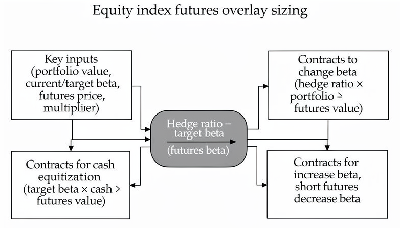 _Equity index futures calculations determine hedge ratios, contract counts for target beta and cash equitization, and exposure direction._ > **Key Term: options overlay** > The use of exchange-traded or OTC options (e.g., calls, puts, or option combinations) applied to a portfolio to manage or limit risk at predetermined price levels while retaining ownership of the cash assets. Compared with futures, options overlays introduce nonlinear payoffs and can create downside protection or upside capping over a specified horizon. Because options are not symmetric, they are particularly useful for clients who care more about limiting losses than about limiting gains. > **Key Term: protective put** > A risk management strategy in which an investor who holds a long position in an asset buys a put option on that asset to establish a minimum sale price (floor) over the option’s life. > **Key Term: covered call** > A strategy in which an investor holds a long position in an asset and sells (writes) a call option on that asset, generating option premium income while capping upside beyond the call strike. > **Key Term: collar** > An options strategy combining a long put and a short call on the same reference asset and maturity, designed to limit downside risk below the put strike while giving up upside beyond the call strike. > **Key Term: delta** > The sensitivity of an option’s price to a small change in the price of the reference asset; interpreted as the approximate hedge ratio between option contracts and asset exposure. > **Key Term: vega** > The sensitivity of an option’s price to a small change in the implied volatility of the reference asset; important when assessing how changes in volatility affect option overlay values. ### Futures vs Options Overlays: Conceptual Contrast For exam purposes, it helps to remember: - Futures overlays - Linear payoff: gains and losses move one‑for‑one with the reference asset (adjusted for hedge ratio). - Primary role: change the quantity of exposure (beta, duration, asset weight). - Symmetric: downside and upside are adjusted similarly. - Require margin; no upfront premium. - Exposure is obligatory: when the futures expires, the payoff happens automatically (cash or physical settlement). - Options overlays - Nonlinear payoff: asymmetric downside vs upside (convexity). - Primary role: change the quality of exposure (downside protection, upside participation). - Useful when the client’s utility is strongly concave for losses (capital preservation priority). - Buyer pays premium; seller receives premium but assumes potentially large obligations. - Exposure is discretionary: the option holder chooses whether to exercise. When asked to “compare and contrast futures and options overlays,” an effective answer will: - Link futures to beta or duration adjustments and tracking error control. - Link options to loss‑limiting and payoff‑shaping objectives. - Discuss cost (premium vs margin), convexity, and suitability for different investor profiles. For instance: - A wealthy retiree worried about a large drawdown will often prefer protective puts or collars. - An index fund concerned about cash drag will rely on equity index futures. - A low‑cost passive strategy may avoid options overlays entirely due to premium costs and operational complexity. ### Typical Uses (Options) - Downside risk protection: Purchase puts (protective put) or implement collars to limit losses below a threshold. - Return capping and cost reduction: Sell calls to partially or fully fund puts, thus creating a cost‑effective risk–return corridor. - Enhancing income: Sell covered call options to generate option premium from existing holdings, especially when expecting flat or mildly rising markets. - Expressing tactical views with limited capital at risk: Buy calls to increase upside exposure or buy puts for short‑term downside views without committing large capital. - Volatility positioning: Take long or short volatility exposure (e.g., via straddles or volatility derivatives), though at Level 3 this is typically a secondary consideration relative to risk management. In the options strategies reading, spreads and combinations (bull spreads, bear spreads, straddles) are covered. In overlay contexts: - A collar can be viewed as a type of “vertical spread plus stock” and is the most exam‑relevant combination for portfolio risk management. - A straddle (long call + long put) is more of a volatility bet than a risk‑reduction overlay and would rarely be appropriate for a conservative IPS whose primary goal is loss limitation. You may be asked to explain why a collar is preferable to, say, a long straddle for a client seeking downside protection with limited cost. ### Worked Example 1.6 An equity fund trades at \$50 per share. The manager buys a 6‑month \$48 put for \$1.50 and sells a 6‑month \$54 call for \$1.50. What is the effect of this collar overlay? > **Answer:** > The option premiums net to zero, so this is a zero‑cost collar. The downside is limited because the put gives the right to sell at \$48; losses below \$48 are truncated. The upside is capped because the short call obliges the manager to sell at \$54; gains above \$54 are forfeited. Over the next six months, the investor participates in equity moves between \$48 and \$54, with protection below \$48 and no benefit above \$54. > For exam purposes, you should: > > - State clearly the floor price (48) and ceiling price (54). > - Note explicitly that this is a zero‑cost collar (put premium = call premium). > - Explain the trade‑off between downside protection and forgone upside, and relate it to the client’s risk preference and return requirement. > > **Key Term: zero‑cost collar** > A collar in which the premium paid for the long put is approximately offset by the premium received from the short call, resulting in no material net premium outlay. > **Key Term: debit collar** > A collar where the cost of the long put exceeds the premium received from the short call, so the investor pays net premium in exchange for stronger downside protection or a higher upside cap. > **Key Term: credit collar** > A collar where the premium received from the short call exceeds the cost of the long put, generating a net premium inflow but usually implying a lower downside floor or tighter upside cap. > > - State clearly the floor price (48) and ceiling price (54). > - Note explicitly that this is a zero‑cost collar (put premium = call premium). > - Explain the trade‑off between downside protection and forgone upside, and relate it to the client’s risk preference and return requirement. ### Overlay Construction Steps When designing an options overlay, a Level 3 answer should show both quantitative and qualitative reasoning: - Determine the exposure to protect or modify. - Total portfolio value, or only the risky portion (e.g., equities). - Whether the overlay is full (100%) or partial (e.g., hedge only 50% of equity exposure). - Whether index options are an acceptable proxy for a diversified equity portfolio. - Specify the risk objective. - Maximum acceptable loss over the horizon (e.g., “protect against more than a 10% decline over one year”). - Willingness to cap upside to reduce or eliminate premium outlay. - Whether the focus is on absolute loss (e.g., “do not lose more than \$2 million”) or relative loss (e.g., “limit underperformance vs benchmark”). - Select option types, strikes, and maturities. - Protective put: choose the strike to set the desired floor. - Covered call: choose the call strike that defines the upside you are willing to give up. - Collar: combine both to align with the client’s risk–return preferences over the relevant horizon. - Ensure that option maturity matches or exceeds the risk horizon in the IPS; if not, comment on the need for rolling and the risk that protection expires before the risk window closes. - Evaluate cost and participation. - Premia paid and received, net option cost, and its impact on expected return. - Scenario analysis across a range of asset prices at option expiry. - Whether a zero‑cost or low‑cost collar meets the risk objective; if not, justify paying net premium for a stronger floor (debit collar). - Set hedge ratio (number of contracts). - Use contract value and, if necessary, option delta to size the overlay relative to the exposure you want to protect or modify. - Ensure the chosen hedge ratio is consistent with any derivatives usage limits (e.g., cannot hedge more than 80% of portfolio). In constructed‑response questions, it is common to see a sequence such as: - (i) “State two ways the manager could use options to achieve the client’s objective.” - (ii) “Recommend the most appropriate strategy and justify your choice.” A high‑scoring answer both identifies the strategies (e.g., protective puts and zero‑cost collars) and clearly links the recommendation to the IPS (loss tolerance, premium budget, time horizon). ### Sizing Option Overlays: Contract Count and Delta Because one option contract usually references a fixed notional amount of the reference asset (e.g., \$100 × index level), the raw number of contracts is: $$\text{Contracts (if } \Delta \approx 1\text{)} = \frac{\text{Exposure to be hedged}}{\text{Contract value}}$$ For deep out‑of‑the‑money or shorter‑dated options, delta may be substantially below 1 in magnitude. To approximate the hedge ratio, adjust for delta: $$\text{Contracts} = \frac{\text{Exposure to hedge}}{\text{Contract value} \times |\Delta|}$$ When delta is not given in the vignette, you may assume: - Index options used for broad equity hedging are often near‑the‑money with $\Delta \approx 1$; or - The exam will supply any non‑standard delta explicitly. You might also need to adjust for beta when using index options to hedge a non‑index portfolio—for example, hedge a portfolio with $\beta = 1.2$ using index puts. In such cases, the exposure to hedge is often taken as $\beta_S \times S$ rather than just $S$, reflecting that the portfolio moves more than the index. ### Worked Example 1.7 A portfolio worth \$2 million is to be fully protected from losses below 95% of current value for the next quarter. The fund manager buys at‑the‑money put options on an index with a delta of 1 and a contract size of \$100,000. How many puts are needed? > **Answer:** > Assuming each option provides protection on \$100,000 of index exposure and has delta ≈ 1, the number of contracts is: > > $$> \text{Contracts} = \frac{2{,}000{,}000}{100{,}000} = 20$$ > > The manager buys 20 index put contracts to hedge the full portfolio value. > If instead the options had a delta of 0.5, the number of contracts required would double: > > $$> \text{Contracts} = \frac{2{,}000{,}000}{100{,}000 \times 0.5} = 40$$ > > In an essay answer, you should also: > > - Make clear whether the client accepts the 5% deductible (loss between 100% and 95%). > - Comment that the hedge is only as good as the proxy relationship between the index and the actual portfolio (basis risk). > - Make clear whether the client accepts the 5% deductible (loss between 100% and 95%). > - Comment that the hedge is only as good as the proxy relationship between the index and the actual portfolio (basis risk). ### Worked Example 1.8 A manager runs a \$50 million equity portfolio closely tracking a broad index. To generate additional income over the next three months, the manager considers selling out‑of‑the‑money index calls with strike 5% above the current index level. The index level is 2,000, the call premium is 2% of index value, and the contract multiplier is \$250. How many call contracts should be sold if the manager wants to write calls on 60% of the portfolio value? > **Answer:** > First, determine the notional equity exposure to be covered: > > $$> 0.60 \times 50\,\text{million} = 30\,\text{million}$$ > > Compute the value per index option contract (using the index as proxy): > > $$> 2{,}000 \times 250 = 500{,}000$$ > > Number of contracts: > > $$> \text{Contracts} = \frac{30{,}000{,}000}{500{,}000} = 60$$ > > The manager sells 60 index call contracts. The option premium income is: > > $$> 30{,}000{,}000 \times 0.02 = 600{,}000$$ > > (ignoring time value and transaction costs). This covered call overlay boosts income but caps upside on 60% of the portfolio beyond the call strike. > A good exam answer will explicitly tie this to the IPS: > > - The strategy is suitable when the client is comfortable exchanging some upside for current income, for example a pension fund seeking stable cash flows. > - Overwriting only 60% of the portfolio provides a compromise: 40% remains uncapped, preserving some full upside potential. > - The strategy is suitable when the client is comfortable exchanging some upside for current income, for example a pension fund seeking stable cash flows. > - Overwriting only 60% of the portfolio provides a compromise: 40% remains uncapped, preserving some full upside potential. ### Protective Puts vs Stop‑Loss Orders An exam‑relevant comparison is between buying protective puts and using stop‑loss orders: - Protective puts provide a contractual floor until expiration, regardless of intraday price path, subject only to counterparty risk. - Stop‑loss orders provide no guarantee; they can be triggered by intraday “noise” or may execute at prices far below the stop level in a gap down. - Options protect against adverse price moves but not necessarily against widening credit spreads or volatility changes in other asset classes; stop‑losses are also purely price based but without convexity. Accordingly: - For clients highly focused on capital preservation over a defined horizon, a protective put overlay (or collar) is usually more suitable despite its cost. - For cost‑sensitive clients or where derivative use is constrained, stop‑loss policies might be considered but should be recognized as imperfect substitutes. Your answer should recognise that stop‑loss orders may add trading costs and can force selling at market troughs, whereas options allow the investor to stay invested through volatility with known downside. ### Collars in Practice You should be able to discuss variations: - Zero‑cost collar: Put premium ≈ call premium; no net premium outlay but both downside and upside are constrained. - Debit collar: Put premium > call premium; investor pays net premium for stronger downside protection or higher upside cap. - Credit collar: Put premium \< call premium; investor receives net premium, accepting a lower floor or tighter upside cap. The choice depends on: - The investor’s willingness to pay explicit insurance cost. - The importance of preserving capital versus retaining upside. - The investment horizon relative to option maturity. - Tax considerations, especially for concentrated low‑basis positions where selling would trigger large capital gains. ### Worked Example 1.9 A client holds a \$10 million equity portfolio. She wants to limit potential loss over the next year to at most 15% while giving up gains beyond +20%. At‑the‑money puts with strike at today’s index level cost 5%; 15% out‑of‑the‑money puts cost 2%; 20% out‑of‑the‑money calls yield 2% when written. Propose a suitable collar and compute the net premium. > **Answer:** > The client wants a floor at approximately −15% and a ceiling at +20%. A natural structure is: > > - Buy 15% out‑of‑the‑money puts (floor at −15%). > Sell 20% out‑of‑the‑money calls (cap at +20%). > > The cost per dollar of notional: Put premium = 2%, call premium received = 2%, net premium = 2% − 2% = 0%. > For a \$10 million portfolio, the dollar premiums are: pay \$200,000 for puts and receive \$200,000 for calls. > Net premium = \$0; this is a zero‑cost collar. It achieves the requested floor and ceiling and is appropriate for a capital‑preservation‑oriented client who is willing to surrender upside beyond +20% in exchange for protection. > In the exam you should also note that the client still bears the first 15% of loss (the deductible) and that the collar would need to be rolled if the risk horizon exceeds one year, introducing roll and basis risk around the roll dates. ### Moneyness and Option Selection > **Key Term: moneyness** > A description of the relationship between the current price of the underlying asset and the option’s strike price (e.g., in the money, at the money, out of the money). Moneyness affects both the cost and the protection level: - Deep out‑of‑the‑money puts are cheaper but offer protection only against severe declines. - At‑the‑money puts are more expensive but start protecting almost immediately. - Out‑of‑the‑money calls (used in collars and covered calls) allow some upside before capping gains; higher strikes reduce call premium income. In constructing an overlay, connecting strike choices to the client’s maximum loss tolerance and minimum required upside is a high‑value discussion point. For a very loss‑averse client, deep out‑of‑the‑money puts may not provide sufficient protection even though they are cheaper. ### Volatility, Implied Volatility, and Skew > **Key Term: implied volatility** > The volatility level for the reference asset that, when input into an option pricing model, reproduces the observed market price of the option. > **Key Term: volatility skew** > The pattern in which implied volatilities differ across strike prices for options with the same maturity, often with higher implied volatilities for out‑of‑the‑money puts than for at‑the‑money options or out‑of‑the‑money calls. In many equity index option markets: - Out‑of‑the‑money puts used for downside protection are in high demand, pushing their implied volatility (and hence their premium) above that of at‑the‑money options. - Out‑of‑the‑money calls used in collars or covered call overlays often have lower implied volatilities and therefore provide less premium per unit of notional. This skew implies that pure protective put overlays can be expensive, whereas collars, which sell relatively cheap upside volatility and buy relatively expensive downside volatility, can provide a more cost‑effective compromise. Recognizing this in your discussion of overlay costs demonstrates depth. The skew itself varies over time. Sharp increases in skew (especially rising implied vol for downside puts) often signal rising market concern about downside risk. For a tail‑risk‑focused institutional investor, this might be exactly the time protection is needed—but premia will be high. You should be able to explain that the timing of purchasing protection relative to volatility conditions affects the cost–benefit trade‑off. ### Volatility Derivatives as Tail‑Risk Overlays Beyond plain index options, the curriculum introduces volatility derivatives such as VIX futures and variance swaps. > **Key Term: volatility derivative** > A derivative contract whose underlying is a measure of volatility (such as the VIX index) rather than the level of an equity index, interest rate, or commodity. > **Key Term: VIX** > A commonly used volatility index measuring the market’s expectation of 30‑day volatility of the S&P 500, derived from S&P 500 option prices. > **Key Term: variance swap** > An OTC derivative contract in which one party pays a fixed variance (squared volatility) and receives realized variance over the contract life, or vice versa. Key points: - Volatility tends to spike when equity markets fall, so long volatility positions (long VIX futures, long variance swaps, or long index puts) can act as tail‑risk hedges for equity portfolios. - These hedges are often costly over time because the term structure of volatility futures is frequently in contango and because implied volatility embeds a risk premium. - Compared with a traditional put overlay, volatility derivatives provide a more direct hedge on volatility, which is negatively correlated with equity returns but not perfectly. At Level 3, you might be asked to compare a rolling put strategy with a rolling long VIX futures strategy as tail‑risk overlays, addressing cost, basis risk (variance vs price risk), and operational complexity. The reading emphasises that: - VIX futures rarely move one‑for‑one with spot VIX, especially at longer maturities. - Maintaining a constant‑maturity long VIX position usually requires frequent rolling in contango, leading to negative carry. - Volatility ETPs that track short‑term VIX futures can substantially underperform spot VIX over time due to this roll‑down effect. A good answer will therefore stress that volatility derivatives are specialised tools for institutions willing to accept an ongoing drag on returns in exchange for protection in extreme downside scenarios. ### Worked Example 1.10 A US equity fund worth \$100 million wants protection against severe market stress over the next six months. The manager is considering: - Strategy A: Buy 5% out‑of‑the‑money 6‑month S&P 500 puts costing 3% of notional. - Strategy B: Take a long position in 6‑month VIX futures. The current VIX is 15, the 6‑month futures price is 18, and historical analysis suggests that in severe sell‑offs the VIX spikes to 35–40. The manager estimates that a notional VIX futures position equal to 20% of the equity portfolio would provide an adequate offset if volatility spikes. Explain, in qualitative terms, the main trade‑offs between these two overlays. > **Answer:** > Strategy A (index puts) directly insures against declines in the equity index level. If the market falls more than 5%, the puts move in the money and gains on the options offset losses on the equity portfolio. The cost is explicit and known upfront (3% of notional), and the payoff is relatively transparent. Protection is strongest for large price declines and is independent of the specific path volatility takes, as long as the price drop occurs before option expiry. > Strategy B (long VIX futures) provides indirect protection by profiting from increases in implied volatility that typically accompany equity sell‑offs. If volatility rises from 18 to, say, 35, the VIX futures position generates a gain that can help offset equity losses. However, the hedge is less direct: if equity markets fall without a large volatility spike, or if volatility rises by less than the market expects (already embedded in the futures price), the protection may be weaker than desired. In addition, rolling long VIX futures in contango can generate significant negative carry over time. > In an exam answer, you would conclude that Strategy A offers more precise and transparent price‑level insurance at a known premium cost, suitable for a client with a clearly defined loss limit. Strategy B is more of a macro volatility hedge whose effectiveness depends on volatility–equity co‑movement and the term structure of VIX futures; it may be considered when the investor specifically anticipates a volatility spike and is willing to accept basis risk between volatility and equity losses. ### Option Overlays for Different Investor Types Options overlays are particularly sensitive to investor type and IPS features: - Private wealth clients: Taxation of realized gains and option premia, emotional loss aversion, and legacy holdings matter. Protective puts or collars are often used to protect concentrated positions without triggering capital gains. - Pension funds and insurers: The focus is often on funding ratio or surplus volatility. Equity index puts or collars can be used to limit downside in the return‑seeking portfolio, with cost benchmarked against the value of reduced surplus volatility. - Foundations and endowments: Spending requirements and long horizons mean they can tolerate more volatility; they may use covered calls for income or low‑cost collars during periods of unusually high equity valuations. When answering IPS‑driven questions, link option overlay design to: - Risk objective (capital preservation vs growth). - Time horizon (and whether a rolling program of options will be needed). - Liquidity and premium budget (aversion to large explicit premia might push you towards zero‑cost collars). - Legal and regulatory constraints (e.g., some institutions restrict uncovered option writing). For example, a life insurer’s IPS might: - Allow limited use of long equity index puts to cap downside risk in the surplus portfolio. - Prohibit selling naked puts or calls because they create potentially large liabilities and regulatory capital charges. - Require that any long‑volatility or tail‑risk hedge be evaluated in terms of its impact on solvency capital and surplus volatility. ### Key Practical Considerations Maintaining precise exposure with derivatives overlays is subject to several real‑world frictions that feature frequently in Level 3 vignettes. > **Key Term: basis risk** > The risk that changes in the price of a derivative (e.g., futures contract or index option) will not perfectly offset changes in the value of the hedged portfolio, leading to residual gain or loss. > **Key Term: gap risk** > The risk that the reference asset price moves sharply (gaps) through the hedge levels between rebalancing dates, so that the overlay does not provide the expected protection at all times. > **Key Term: roll risk** > The risk that the cost or effectiveness of a derivative overlay changes unfavourably when positions are rolled from a maturing contract to a later‑dated contract. Key considerations include: - Basis risk - For futures overlays, the portfolio may not perfectly match the index used by the futures (different constituents, sector weights, or beta), so the hedge is imperfect. - For equity options overlays, index options may not match the specific stock mix; moreover, implied volatility may change differently from realized volatility. - For duration overlays, basis risk arises when the yield curve shifts are not parallel, so matching overall duration does not fully hedge key interest rate risks. - For volatility derivatives, the hedge is on implied volatility; realised volatility and equity prices may behave differently than expected. - In exam answers, reference basis risk whenever the actual portfolio is described as “custom,” “concentrated,” or “fundamentally different” from the index referenced by the derivative. - Contract expiry and rolling - Futures and options have finite lives; overlays must be rolled to maintain coverage beyond expiration. - Rolling introduces roll risk: changes in futures basis or option implied volatility can alter hedge cost and effectiveness. - For example, if equity index futures move from backwardation to contango, rolling a long futures overlay becomes more expensive (negative roll yield). - For protective put programs, if implied volatility rises before the roll date, new options will be more expensive, increasing the cost of maintaining the hedge. - Liquidity and transaction costs - Large overlay positions require sufficient depth in the futures or options market. - Bid–ask spreads and commissions reduce effectiveness, especially for options strategies requiring multiple legs or frequent rebalancing. - When comparing overlays vs physical rebalancing, note that overlays often have lower transaction costs per unit of exposure but may involve ongoing roll costs. - Margin requirements and cash management - Futures positions require initial and variation margin; adverse moves can trigger margin calls, creating liquidity risk. - For option overlays, purchased options require upfront premia; written options generate premium but introduce potential future obligations and may require margin if written uncovered. - A well‑structured exam answer will mention whether the investor has sufficient liquidity to meet margin calls or option obligations, especially important for private wealth clients with limited liquid reserves. - Operational and monitoring complexity - Overlays require robust risk systems for monitoring exposures, marking to market, and ensuring compliance with investment guidelines. - Mis‑sizing hedges, failing to roll contracts, or misaligning maturities are common operational issues. - Governance arrangements (investment committees, ALM committees) should be adequate to control model risk and execution risk. - Option market conditions: volatility level and skew - Protective puts (out‑of‑the‑money downside puts) are often in high demand, increasing their implied volatility relative to at‑the‑money options and out‑of‑the‑money calls. - This volatility skew makes pure put‑based protection relatively expensive; collars (selling calls to help pay for puts) can be a more cost‑effective compromise. - Recognizing and citing volatility skew as a reason why protective puts may be costly is a high‑quality Level 3 response. - Use of volatility derivatives as overlays - Some institutional investors use long volatility exposure (e.g., via volatility futures or variance swaps) as a tail‑risk hedge overlay on equity portfolios. - These strategies can be compared with traditional options overlays, considering cost, convexity, and basis risk relative to the actual portfolio. - Because long volatility strategies may suffer from negative carry in normal markets, the IPS should clarify whether the client is willing to pay this ongoing insurance cost. - Regulatory and accounting treatment - For institutions (banks, insurers, pensions), the treatment of derivatives under solvency and accounting rules can affect the attractiveness of overlays. - For example, some regulators may require additional capital for options sold, or may treat certain derivatives as increasing leverage, affecting risk‑based capital ratios. - In exam questions about institutional investors, tie overlay recommendations to these regulatory and accounting considerations where relevant. From the banking and insurance readings, you should recall that: - Banks and insurers often manage assets and liabilities on an economic (mark‑to‑market) basis even though accounting and regulatory capital calculations may smooth earnings. - Derivatives overlays are frequently used by bank treasury and CIO functions to manage interest‑rate risk and foreign‑exchange risk on the balance sheet. - ALM or investment committees set the overall IPS, including permitted derivatives, collateral management, and reporting requirements. When evaluating an overlay for a bank or insurer, mention: - Impact on liquidity ratios and regulatory stress tests. - Interaction with statutory accounting (e.g., unrealised gains/losses on derivatives). - Whether the proposed overlay fits within the institution’s enterprise risk management framework. ### Overlays vs Physical Rebalancing A common exam task is to compare implementing a view via derivatives overlays versus physical trades. - Overlays are generally preferable when: - The desired exposure change is temporary (tactical view). - Existing holdings are illiquid, tax‑sensitive, or carry embedded gains the client wishes to defer. - The portfolio is large and diversified, making physical rebalancing slow and expensive. - The investor wants to separate alpha from beta (e.g., maintain stock selection positions while neutralizing market risk with futures). - The adjustment required is small relative to portfolio size and within tactical bands, and the manager wants to avoid unnecessary turnover. - The investor values capital efficiency, keeping more assets invested in return‑seeking strategies rather than tied up in cash. - Physical rebalancing may be preferable when: - The change in allocation is strategic and long term, making ongoing roll costs unattractive. - The investor wants to reduce not only systematic risk but also idiosyncratic risk of specific holdings (e.g., sell concentrated stock positions). - There are binding constraints on derivatives usage or leverage. - The portfolio manager wants to simplify governance and reduce operational complexity. - The portfolio holds assets with limited derivative proxies, making overlay hedges ineffective or impractical. - Liquidity in the relevant futures or options market is limited, increasing implementation risk. When asked to “recommend and justify” an approach, tie your answer to: - Investment horizon (temporary vs permanent change). - Tax and transaction cost implications. - Liquidity and market impact. - Client tolerance for complexity and leverage. - Regulatory or accounting considerations for institutional investors. You should also link the choice to business‑cycle expectations. Because the cycle signal is noisy, using a highly leveraged overlay to express a macro view is rarely appropriate for conservative institutions. Instead, moderate overlay sizes within IPS tactical bands, combined with clear time horizons and review triggers, are more defensible. ### Risk and Limitations Derivatives overlays are powerful but imperfect tools. At Level 3, you must critically evaluate whether an overlay is appropriate and what residual risks remain. - Imperfect hedges - Portfolio beta and duration are estimates that can change over time; if these parameters drift, the initial hedge ratio may no longer be appropriate. - Using a single index futures contract to hedge a multi‑asset or style‑tilted portfolio will not eliminate all systematic risk. - For options, discrete strikes and maturities restrict how precisely you can match the desired payoff; path dependency and early exercise (for American options) may also matter. - For volatility derivatives, the hedge is on volatility, not directly on price; sharp declines in equities that are not accompanied by large volatility spikes may leave residual risk. - Gearing and leverage effects - Futures overlays create leverage because relatively small margin amounts control large notional exposures. - This can magnify both gains and losses; if poorly sized, overlays can create risk that exceeds the investor’s tolerance or regulatory limits. - Writing options (especially naked puts or calls) also embeds leverage and short‑volatility exposure; losses can be substantial in extreme market moves. - In an IPS context, derivatives overlays should be explicitly recognised as potential sources of leverage, and position limits should reflect this. - Model and parameter risk - Mis‑estimating beta, duration, or option delta leads to over‑ or under‑hedging. - Volatility assumptions matter for options pricing and for evaluating the cost–benefit of protective strategies. - In fixed income, errors in estimating key rate duration and yield curve movements can cause duration overlays to underperform expectations. - Over‑reliance on historical correlations (for basis risk) can be dangerous if market regimes shift, especially around business‑cycle turning points. - Counterparty and credit risk - Exchange‑traded futures and options have minimal counterparty risk due to central clearing and margining. - OTC options and variance swaps involve counterparty exposure; collateral, netting agreements, and legal documentation (e.g., ISDA) are relevant, especially in institutional contexts. - For insurers and banks, counterparty exposure is often tightly regulated; the IPS will typically set minimum credit‑quality standards for derivative counterparties. - Gap risk and path dependency - Options overlays only guarantee payoffs at or before expiration; large intra‑period moves can cause mark‑to‑market losses that exceed expectations, especially for strategies like covered calls or short puts. - Dynamic hedging strategies (e.g., frequent rebalancing of delta‑hedged positions) are sensitive to price paths and transaction costs. - For portfolios funded with leverage, adverse market gaps can trigger margin calls and forced deleveraging before the options maturity is reached. - Constraints and governance - Some investment policies restrict or prohibit derivatives use, or limit the proportion of portfolio exposure that can be implemented synthetically. - Derivatives overlays may affect reported tracking error, risk measures, or compliance with regulatory limits (e.g., UCITS, ERISA). - The IPS should state clearly whether overlays are permitted and within what ranges. - Governance bodies (investment committees, ALM committees) should monitor overlay programs, including stress tests and scenario analysis. ### Exam Warning and Answer Construction Many candidates incorrectly assume that a futures or options overlay completely eliminates risk. In practice, overlays are subject to basis risk, model error, gap risk, and expiration mismatch. In constructed‑response answers, always identify at least one residual risk and briefly explain its source. This demonstrates a realistic understanding of derivatives rather than a purely theoretical one. A robust Level 3 answer to an overlay question typically has three components: - **Calculation:** Correctly compute the number of contracts or the hedge ratio, showing your formula and substituting numbers clearly. - **Interpretation:** Explain in words what the overlay does to portfolio beta, duration, or payoff profile, and how it affects tracking error or surplus volatility. - **IPS and governance linkage:** Comment on whether the overlay is consistent with the client’s risk objectives, constraints (including derivative limits), liquidity profile, and business‑cycle view. Time management matters: for a 6‑point constructed‑response sub‑question, two or three precise sentences after the calculation are normally sufficient, provided they address these elements explicitly. ## Summary Derivative overlays using futures and options are key tools in portfolio risk management at Level 3. By overlaying positions, managers can: - Adjust equity beta or bond duration rapidly. - Implement tactical asset allocation views without disturbing long‑term holdings. - Control downside risk and shape payoff patterns through protective puts, covered calls, and collars. - Equitize cash to minimize tracking error relative to benchmarks. - Align asset sensitivity (beta, duration) with liability characteristics in institutional portfolios. - Implement tail‑risk hedges using index options or volatility derivatives. However, overlays carry limitations such as basis risk, imperfect hedges, leverage, and additional operational complexity. Futures overlays are linear and primarily adjust quantity of exposure (beta, duration), whereas options overlays are nonlinear and adjust quality of exposure (downside protection vs upside participation). Effective exam answers combine correct calculations (number of contracts, hedge ratios) with clear qualitative explanations of objectives, trade‑offs, and implementation risks—and always relate the chosen overlay to the client’s IPS, business‑cycle view, and governance framework. ## Key Point Checklist _This article has covered the following key knowledge points:_ - Understand objectives and methods of futures and options overlays in portfolio risk management. - Calculate required futures or options contracts to adjust exposure or achieve hedges, including beta overlays, duration overlays, and cash equitization. - Identify and explain typical uses of overlays—tactical asset allocation, cash equitization, risk reduction, income enhancement, tail‑risk hedging, and asset–liability alignment. - Evaluate main risks—basis risk, transaction cost, contract expiry, gearing effects, gap risk, volatility skew, and roll risk—and how these impact overlay effectiveness. - Compare overlays with outright buying, selling, or physical rebalancing approaches and justify implementation choices in exam scenarios. - Integrate qualitative reasoning with quantitative calculations to construct clear constructed‑response answers on derivatives overlays. - Recognize when options overlays (protective puts, covered calls, collars) are more appropriate than futures overlays, given client risk preferences and constraints. - Appreciate how volatility derivatives (VIX futures, variance swaps) can complement options overlays as tail‑risk hedges, and assess their costs and basis risks. - Relate overlay decisions explicitly to IPS elements such as risk objectives, liquidity needs, tax considerations, and derivatives constraints. - Link tactical overlay decisions to business‑cycle expectations while acknowledging the uncertainty and noise in macro timing signals. ## Key Terms and Concepts - derivatives overlay - hedge ratio - tracking error - tail‑risk hedge - futures overlay - contract multiplier - beta overlay - cash equitization - duration overlay - basis point value (BPV) - cheapest to deliver (CTD) - surplus optimization - hedging/return‑seeking portfolios approach - contango - backwardation - roll yield - options overlay - protective put - covered call - collar - delta - vega - zero‑cost collar - debit collar - credit collar - moneyness - implied volatility - volatility skew - volatility derivative - VIX - variance swap - basis risk - gap risk - roll risk